On this page we take the topology examples previously introduced on the page here and go on to relate this to the homology of these examples.
Now we continue with the square example above but this time we treat it as a solid square. The mapping from edge to vertices is the same as above but now we also have a mapping from square to edges.
| In order to represent the homology from this we need to have each mapping indexing into the next. | 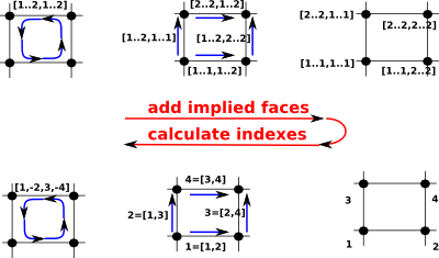 |
So, on the above diagram going across the top row, starting from the square [1..2,1..2] we can generate all possible edges:
and from them we can generate all possible vertices:
Then, going left across the bottom row, we can replace these with indexes so that each dimension indexes into the next. |
(1) -> ACUBE := FiniteCubicalComplex(Integer)

   (1)  FiniteCubicalComplex(Integer)
                                     Type: Type
(2) -> vs1:List(Integer) := [1,2,3,4]

   (2)  [1,2,3,4]
                            Type: List(Integer)
(3) -> sp := sphereSolid(2)$CubicalComplexFactory

   (3)
        (1..2,1..2)
            Type: FiniteCubicalComplex(Integer)
(4) -> d5 := sp::DeltaComplex(Integer)

   (4)
                  2D:[[- 1,4,2,- 3]]
         1D:[[- 1,2],[- 1,3],[- 2,4],[- 3,4]]
                 0D:[[0],[0],[0],[0]]
Type: DeltaComplex(Integer) |
Conversion to Chain Complex
Now we have the delta complex we can go on to generate a 'chain complex', this consists of a sequence of matrices which map each array of indices to the next higher array.
I have put a more general discussion of chain complexes on page here.
Once we have added the implied faces we can then give each vertex an index number. The index numbers, for each square, need not be consecutive as in the diagram but:
|
 |
|||||||||||||||||
We can now map to a set of indexes for the edges as follows:
|
|
|||||||||||||||||
| This gives indexes for the edges as shown on the diagram on the right: |  |
|||||||||||||||||
|
||||||||||||||||||
 |
||||||||||||||||||
This matrix defines the mapping Note: the edges are not numbered in the order that we travel around the square, that would be: 1,2,-4,-3. |
square |
|||
| edges | [1..2,1..2] |
|||
| 1 =[1..2,1..1] | +1 |
|||
| 2 =[2..2,1..2] | +1 |
|||
| 3 = -[1..1,1..2] | -1 |
|||
| 4 = -[1..2,2..2] | -1 |
|
(5) -> chain(d5)

                     +- 1  - 1   0    0 + +- 1+
                     | 1    0   - 1   0 | | 1 |
   (5)  [0  0  0  0],|                  |,|   |,[]
                     | 0    1    0   - 1| |- 1|
                     + 0    0    1    1 + + 1 +
                             Type: ChainComplex
(6) -> homology(sp)

   (6)  [Z,0,0]
Type: List(Homology) |
Another Example - Connected
If we add more squares like this: |
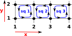 |
| Then we get more columns in the matrix. | squares
|
|||||
| edges | [1..2,1..2] |
[2..3,1..2] |
[3..4,1..2] |
|||
| [1..2,1..1] | +1 |
0 |
0 |
|||
| [2..2,1..2] | +1 |
+1 |
+1 |
|||
| -[1..2,2..2] | -1 |
0 |
0 |
|||
| -[1..1,1..2] | -1 |
-1 |
-1 |
|||
| [2..3,1..1] | 0 |
+1 |
0 |
|||
| [3..4,1..1] | 0 |
0 |
+1 |
|||
| -[3..4,2..2] | 0 |
0 |
-1 |
|||
| -[2..3,2..2] | 0 |
-1 |
0 |
|||
In FriCAS we can run as follows: First we setup the cubical complex as described on previous page. |
(7) -> Sq1 := cubicalFacet(1,[1..2,1..2])

   (7)  (1..2,1..2)
                             Type: CubicalFacet
(8) -> Sq2 := cubicalFacet(1,[2..3,1..2])

   (8)  (2..3,1..2)
                             Type: CubicalFacet
(9) -> Sq3 := cubicalFacet(1,[3..4,1..2])

   (9)  (3..4,1..2)
                             Type: CubicalFacet
(10) -> ex1:=cubicalComplex(vs1,[Sq1,Sq2,Sq3])$ACUBE

   (10)
         (1..2,1..2)
         (2..3,1..2)
         (3..4,1..2)
            Type: FiniteCubicalComplex(Integer)
(11) -> boundary(ex1)

   (11)
         -(1..1,1..2)
         (1..2,1..1)
         -(1..2,2..2)
         (2..3,1..1)
         -(2..3,2..2)
         (4..4,1..2)
         (3..4,1..1)
         -(3..4,2..2)
Type: FiniteCubicalComplex(Integer |
We can coerce this into a DeltaComplex which indexes each dimension into the next lower. DeltaComplex is used internally for calculating chain and homology. |
(12) -> d3 := ex1::DeltaComplex(Integer)

   (12)
   VCONCAT
      VCONCAT
          2D:[[- 1,4,2,- 3],[- 4,7,5,- 6],[- 7,10,8,- 9]]
     ,
          1D:
           [[- 1,2], [- 1,3], [- 2,4], [- 3,4], [- 3,5], [- 4,6], [- 5,6],
            [- 5,7], [- 6,8], [- 7,8]]
  ,
       0D:[[0],[0],[0],[0],[0],[0],[0],[0]]
Type: DeltaComplex(Integer) |
| The chain is matrix which goes from edges to to vertices. | (13) -> chain(d3)
(13)
+- 1 - 1 0 0 0 0 0 0 0 0 +
| 1 0 - 1 0 0 0 0 0 0 0 |
| 0 1 0 - 1 - 1 0 0 0 0 0 |
| 0 0 1 1 0 - 1 0 0 0 0 |
[0 0 0 0 0 0 0 0],| |
| 0 0 0 0 1 0 - 1 - 1 0 0 |
| 0 0 0 0 0 1 1 0 - 1 0 |
| 0 0 0 0 0 0 0 1 0 - 1|
+ 0 0 0 0 0 0 0 0 1 1 +
,
+- 1 0 0 +
| 1 0 0 |
|- 1 0 0 |
| 1 - 1 0 |
| | ++
| 0 1 0 | ||
| |,||
| 0 - 1 0 | ||
| | ++
| 0 1 - 1|
| 0 0 1 |
| 0 0 - 1|
+ 0 0 1 +
Type: ChainComplex |
| Homology is connected space with no holes. | (14) -> homology(ex1)
(14) [Z,0,0]
Type: List(Homology) |
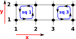
Another Example - Not Connected
This time the squares don't connect to each other : |
 |
In FriCAS we can run as follows: First we setup the cubical complex as described on previous page. |
(15) -> ex2:=cubicalComplex(vs1,[Sq1,Sq2,Sq3])$ACUBE

   (15)
         (1..2,1..2)
         (2..3,1..2)
         (3..4,1..2)
            Type: FiniteCubicalComplex(Integer)
(16) -> boundary(ex2)

   (16)
         -(1..1,1..2)
         (1..2,1..1)
         -(1..2,2..2)
         (2..3,1..1)
         -(2..3,2..2)
         (4..4,1..2)
         (3..4,1..1)
         -(3..4,2..2)
            Type: FiniteCubicalComplex(Integer)
|
We can coerce this into a DeltaComplex which indexes each dimension into the next lower. DeltaComplex is used internally for calculating chain and homology. |
(17) -> d32 := ex2::DeltaComplex(Integer)

   (17)
   VCONCAT
      VCONCAT
          2D:[[- 1,4,2,- 3],[- 4,7,5,- 6],[- 7,10,8,- 9]]
     ,
          1D:
           [[- 1,2], [- 1,3], [- 2,4], [- 3,4], [- 3,5], [- 4,6], [- 5,6],
            [- 5,7], [- 6,8], [- 7,8]]
  ,
       0D:[[0],[0],[0],[0],[0],[0],[0],[0]]
Type: DeltaComplex(Integer) |
| The chain is matrix which goes from edges to to vertices. | (18) -> chain(d32)
(18)
+- 1 - 1 0 0 0 0 0 0 0 0 +
| 1 0 - 1 0 0 0 0 0 0 0 |
| 0 1 0 - 1 - 1 0 0 0 0 0 |
| 0 0 1 1 0 - 1 0 0 0 0 |
[0 0 0 0 0 0 0 0],| |
| 0 0 0 0 1 0 - 1 - 1 0 0 |
| 0 0 0 0 0 1 1 0 - 1 0 |
| 0 0 0 0 0 0 0 1 0 - 1|
+ 0 0 0 0 0 0 0 0 1 1 +
,
+- 1 0 0 +
| 1 0 0 |
|- 1 0 0 |
| 1 - 1 0 |
| | ++
| 0 1 0 | ||
| |,||
| 0 - 1 0 | ||
| | ++
| 0 1 - 1|
| 0 0 1 |
| 0 0 - 1|
+ 0 0 1 +
Type: ChainComplex |
| This time the space is not connected. | (19) -> homology(ex2)
(19) [Z,0,0]
Type: List(Homology) |
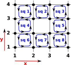
Another Example - Squares with Hole
This time we leave a hole in the array of squares: |
 |
In FriCAS we can run as follows: First we setup the cubical complex as described on previous page. |
(20) -> Sq1 := cubicalFacet(1,[1..2,1..2])

   (20)  (1..2,1..2)
                             Type: CubicalFacet
(21) -> Sq2 := cubicalFacet(1,[2..3,1..2])

   (21)  (2..3,1..2)
                             Type: CubicalFacet
(22) -> Sq3 := cubicalFacet(1,[3..4,1..2])

   (22)  (3..4,1..2)
                             Type: CubicalFacet
(23) -> Sq4 := cubicalFacet(1,[1..2,2..3])

   (23)  (1..2,2..3)
                             Type: CubicalFacet
(24) -> Sq5 := cubicalFacet(1,[3..4,2..3])

   (24)  (3..4,2..3)
                             Type: CubicalFacet
(25) -> Sq6 := cubicalFacet(1,[1..2,3..4])

   (25)  (1..2,3..4)
                             Type: CubicalFacet
(26) -> Sq7 := cubicalFacet(1,[2..3,3..4])

   (26)  (2..3,3..4)
                             Type: CubicalFacet
(27) -> Sq8 := cubicalFacet(1,[3..4,3..4])

   (27)  (3..4,3..4)
                             Type: CubicalFacet
(28) -> sq1:=cubicalComplex(vs1,_
     [Sq1,Sq2,Sq3,Sq4,Sq5,Sq6,Sq7,Sq8])$ACUBE

   (28)
         (1..2,1..2)
         (2..3,1..2)
         (3..4,1..2)
         (1..2,2..3)
         (3..4,2..3)
         (1..2,3..4)
         (2..3,3..4)
         (3..4,3..4)
            Type: FiniteCubicalComplex(Integer)
(29) -> boundary(sq1)

   (29)
         -(1..1,1..2)
         (1..2,1..1)
         (2..3,1..1)
         -(2..3,2..2)
         (4..4,1..2)
         (3..4,1..1)
         -(1..1,2..3)
         (2..2,2..3)
         -(3..3,2..3)
         (4..4,2..3)
         -(1..1,3..4)
         -(1..2,4..4)
         (2..3,3..3)
         -(2..3,4..4)
         (4..4,3..4)
         -(3..4,4..4)
Type: FiniteCubicalComplex(Integer) |
We can coerce this into a DeltaComplex which indexes each dimension into the next lower. DeltaComplex is used internally for calculating chain and homology. |
(30) -> d3 := sq1::DeltaComplex(Integer)

   (30)
   VCONCAT
      VCONCAT
         VCONCAT
        ,
             2D:
              [[- 1,8,4,- 5], [- 2,9,5,- 6], [- 3,10,6,- 7], [- 8,15,11,- 12],
               [- 10,17,13,- 14], [- 15,22,18,- 19], [- 16,23,19,- 20],
               [- 17,24,20,- 21]]
     ,
          1D:
           [[- 1,2], [- 2,3], [- 3,4], [- 1,5], [- 2,6], [- 3,7], [- 4,8],
            [- 5,6], [- 6,7], [- 7,8], [- 5,9], [- 6,10], [- 7,11], [- 8,12],
            [- 9,10], [- 10,11], [- 11,12], [- 9,13], [- 10,14], [- 11,15],
            [- 12,16], [- 13,14], [- 14,15], [- 15,16]]
  ,
       0D:[[0],[0],[0],[0],[0],[0],[0],[0],[0],[0],[0],[0],[0],[0],[0],[0]]
                    Type: DeltaComplex(Integer)
|
| The chain is matrix which goes from edges to to vertices. | (31) -> chain(d3)
(31)
[0 0 0 0 0 0 0 0 0 0 0 0 0 0 0 0]
,
[[- 1,0,0,- 1,0,0,0,0,0,0,0,0,0,0,0,0,0,0,0,0,0,0,0,0],
[1,- 1,0,0,- 1,0,0,0,0,0,0,0,0,0,0,0,0,0,0,0,0,0,0,0],
[0,1,- 1,0,0,- 1,0,0,0,0,0,0,0,0,0,0,0,0,0,0,0,0,0,0],
[0,0,1,0,0,0,- 1,0,0,0,0,0,0,0,0,0,0,0,0,0,0,0,0,0],
[0,0,0,1,0,0,0,- 1,0,0,- 1,0,0,0,0,0,0,0,0,0,0,0,0,0],
[0,0,0,0,1,0,0,1,- 1,0,0,- 1,0,0,0,0,0,0,0,0,0,0,0,0],
[0,0,0,0,0,1,0,0,1,- 1,0,0,- 1,0,0,0,0,0,0,0,0,0,0,0],
[0,0,0,0,0,0,1,0,0,1,0,0,0,- 1,0,0,0,0,0,0,0,0,0,0],
[0,0,0,0,0,0,0,0,0,0,1,0,0,0,- 1,0,0,- 1,0,0,0,0,0,0],
[0,0,0,0,0,0,0,0,0,0,0,1,0,0,1,- 1,0,0,- 1,0,0,0,0,0],
[0,0,0,0,0,0,0,0,0,0,0,0,1,0,0,1,- 1,0,0,- 1,0,0,0,0],
[0,0,0,0,0,0,0,0,0,0,0,0,0,1,0,0,1,0,0,0,- 1,0,0,0],
[0,0,0,0,0,0,0,0,0,0,0,0,0,0,0,0,0,1,0,0,0,- 1,0,0],
[0,0,0,0,0,0,0,0,0,0,0,0,0,0,0,0,0,0,1,0,0,1,- 1,0],
[0,0,0,0,0,0,0,0,0,0,0,0,0,0,0,0,0,0,0,1,0,0,1,- 1],
[0,0,0,0,0,0,0,0,0,0,0,0,0,0,0,0,0,0,0,0,1,0,0,1]]
,
+- 1 0 0 0 0 0 0 0 +
| 0 - 1 0 0 0 0 0 0 |
| 0 0 - 1 0 0 0 0 0 |
| 1 0 0 0 0 0 0 0 |
|- 1 1 0 0 0 0 0 0 |
| 0 - 1 1 0 0 0 0 0 |
| 0 0 - 1 0 0 0 0 0 |
| 1 0 0 - 1 0 0 0 0 |
| 0 1 0 0 0 0 0 0 | ++
| 0 0 1 0 - 1 0 0 0 | ||
| 0 0 0 1 0 0 0 0 | ||
| 0 0 0 - 1 0 0 0 0 | ||
| |,||
| 0 0 0 0 1 0 0 0 | ||
| 0 0 0 0 - 1 0 0 0 | ||
| 0 0 0 1 0 - 1 0 0 | ||
| 0 0 0 0 0 0 - 1 0 | ++
| 0 0 0 0 1 0 0 - 1|
| 0 0 0 0 0 1 0 0 |
| 0 0 0 0 0 - 1 1 0 |
| 0 0 0 0 0 0 - 1 1 |
| 0 0 0 0 0 0 0 - 1|
| 0 0 0 0 0 1 0 0 |
| 0 0 0 0 0 0 1 0 |
+ 0 0 0 0 0 0 0 1 +
Type: ChainComplex |
| This time the space is not connected. | (32) -> homology(sq1)
(32) [Z,Z,0]
Type: List(Homology) |