Delta Complexes Code

We looked at the SimpectialComplex on the previous page. Delta complexes give us an alternative way to encode topological structures. The difference is that the boundary of delta complexes does not have to have distinct faces, for instance, an edge can go from a point back to the same point. We also represent them differently, each dimension indexes into the dimension below it rather than everything being indexed into points as with simplectial complexes.

The dimension of a simplex no loger depends on the number of points in the simplex. So a delta complex can be created from any type of cell complex (no longer just triangles but also squares ...) or a mixture of them.

Advantages of Simpectial Complexes

Easier to construct and to understand
Some operations are easier on simplectial complexes.

Advantages of Delta Complexes

Can sometimes be more compact, for example, use less points.
Easier to contstuct chains, homology and homotopy from delta complexes so they are a good intermediate step.

So it is worthwhile implementing both types in code with conversions between them.

It is possible to convert from and to simpectial complexes like this:

simpectial complexes ->  delta complexes -> simpectial complexes

and get back to where we started. However it is not always possible to start with delta complexes and get back to where we started.

delta complexes -> simpectial complexes ->  delta complexes

This is because the more compact coding of delta complexes is hard to translate because it can only be done by adding extra points. Also the two types are not exactly isomorphic as there are special cases which can only be coded in one type.

There are also other codings of cell complexes such as cubical complexes, we will discuss these on further pages.

Three types of cell complex are implemented:

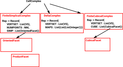Delta Complex

When we looked at the delta complex we got a chain of 'face maps' between each dimension and the next lower one.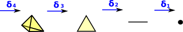

In homology we treat this as a chain of abelian groups (more detail on the page here).

The above representation defines faces, of any dimension, by their vertices. This is an efficient way to define them, the only disadvantage is that intermediate parts, such as edges, are not indexed. It is sometimes useful to be able to do this, for example, when generating homotopy groups such as the fundamental group.

To do this we represent the complex as a sequence of 'face maps' each one indexed into the next.

The ordering of the indexes is important. The indexes of any face are always ordered acording to their order in the next order face.

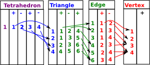
As an example consider the representation for a single tetrahedron:

The usual representation would be:	(1,2,3,4)
which is very efficient but it does not allow us to refer to its edges and triangles.
Here we have indexed: The 4 vertices (in red) The 6 edges (in green) The 4 triangles (in blue)
This representation holds all these indexes so that we don't have to keep creating them and they can be used consistently.
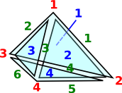
Face Maps So the tetrahedron indexes its 4 triangles, each triangle indexes its 3 edges and each edge indexes its 2 vertices. Each face table therefore indexes into the next. To show this I have drawn some of the arrows (I could not draw all the arrows as that would have made the diagram too messy).

Since edges, triangles, tetrahedrons, etc. are oriented we need to put the indexed in a certain order.

Edges are directed in the order of the vertex indices. That is low numbered index to high numbered index: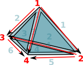
For triangles we go in the order of the edges, except the middle edge is reversed. On the diagram the edges are coloured as follows: green arrows - not reversed purple arrows - reversed This gives the triangles a consistent winding
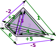However the whole tetrahedron is not yet consistent because some adjacent edges go in the same direction and some go in opposite directions.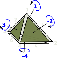
This gives the orientation of the faces as given by the right hand rule. That is: if the thumb of the right hand is outside the tetrahedion, pointing toward the face, then the fingers tend to curl round in the direction of the winding.

The higher order faces may continue on in this manor, however it is difficult to visualize.

So to represent this structure we use the following:

Rep := Record(VERTS:VS,SIMP:List(List(Integer)))

where:

VS is a list of verticies in whatever form we are using.
Integer is an index, a negative sign reverses the direction.
The inner list represents one of the tables shown above, edge has 2 entries, triangle has 3, and so on.
The outer list holds all the tables, edge first, then triangles and so on.

Creating Delta Complexes

Here are 3 ways to construct a delta complex:

From DeltaComplexFactory - Some simple complexes are provided by factory functions.

We cab easily construct from factory functions like this:

(5) -> cD := circle()$DeltaComplexFactory(Integer)

   (5)
         1D:[[1,- 1]]
           0D:[[0]]
                               Type: DeltaComplex(Integer)

From FiniteSimplicialComplex - Sometimes it is easier to construct a simplicial complex first and then convert.

Constructing from a simplicial complex first and then converting:

(6) -> cS := sphereSurface(2)$SCF

   (6)  points 1..3
           (1,2)
          -(1,3)
           (2,3)
                   Type: FiniteSimplicialComplex(Integer)
(7) -> deltaComplex(cS)

   (7)
         1D:[[1,- 2],[- 1,3],[2,- 3]]
               0D:[[0],[0],[0]]
                               Type: DeltaComplex(Integer)

Directly from index lists.

Here we construct directly from index lists:

(8) -> deltaComplex([],1, [[[1, -1]]])$DeltaComplex(Integer)

   (8)
          1D:[[1,- 1]]
            0D:[[0]]
                               Type: DeltaComplex(Integer)

Representation of Delta Complexes

The representation consists of:

vertexset - As for simpectial complex.
maps - Highest dimension first down to dimension zero (points)

The array for each point is either [0] for a used point or [] for an unused point. By 'unused point' I mean a point that is not part of this delta complex but its position is held for future use.

Examples

Here is an example of a tetrahedron (2-sphere).

First we setup 'factories' for DeltaComplex and SimplicialComplex then we convert a SimplicialComplex solid sphere to a DeltaComplex.

(1) -> DCF := DeltaComplexFactory(Integer)

   (1)  DeltaComplexFactory(Integer)
                                               Type: Type
(2) -> SCF := SimplicialComplexFactory(Integer)

   (2)  SimplicialComplexFactory(Integer)
                                               Type: Type
(3) -> sphere := sphereSolid(3)$SCF

   (3)  points 1..4
         (1,2,3,4)
                   Type: FiniteSimplicialComplex(Integer)
(4) -> csphere := deltaComplex(sphere)

   (4)
                          3D:[[1,- 2,3,- 4]]
             2D:[[1,- 2,4],[1,- 3,5],[2,- 3,6],[4,- 5,6]]
         1D:[[1,- 2],[1,- 3],[1,- 4],[2,- 3],[2,- 4],[3,- 4]]
                         0D:[[0],[0],[0],[0]]
                              Type: DeltaComplex(Integer)

Other Examples

Here we constuct a varoius shapes, using factories created above, first directly as a delta then convert from simplex to compare results.

Unconnected Points

This tests that unconnected points are handled correctly.

This example has 4 points:

point 1 and 2 are endpoins of a line.
point 3 does not exist but we want to reserve the index.
point 4 exist but is not connected to anything.

We want to test that this is correctly converted to a delta complex.

(20) -> ASIMP := FiniteSimplicialComplex(Integer)

   (20)  FiniteSimplicialComplex(Integer)
                                               Type: Type
(21) -> v1:List(List(NNI)) := [[1::NNI,2::NNI],[4::NNI]]

   (21)  [[1,2],[4]]
                     Type: List(List(NonNegativeInteger))
(22) -> sc1 := simplicialComplex([],4,v1)$ASIMP

   (22)  points 1..4
            (1,2)
             (4)
                   Type: FiniteSimplicialComplex(Integer)
(23) -> d1 := deltaComplex(sc1)

   (23)
             1D:[[1,- 2]]
          0D:[[0],[0],[],[0]]
                              Type: DeltaComplex(Integer)

Circle

More about topology of circle on page here.

Constuct a circle first directly as a delta then convert from simplex.

The first delta representation is much simpler as it allows us to use only one point.

(5) -> cD := circle()$DCF

   (5)
         1D:[[1,- 1]]
           0D:[[0]]
                               Type: DeltaComplex(Integer)
(6) -> cS := sphereSurface(2)$SCF

   (6)  points 1..3
           (1,2)
          -(1,3)
           (2,3)
                   Type: FiniteSimplicialComplex(Integer)
(7) -> deltaComplex(cS)

   (7)
         1D:[[1,- 2],[- 1,3],[2,- 3]]
               0D:[[0],[0],[0]]
                               Type: DeltaComplex(Integer)

Dunce Hat

Constuct a dunce hat first directly as a delta then convert from simplex.

Again the first delta representation is much simpler using one point.

(8) -> dhD := dunceHat()$DCF

   (8)
         2D:[[1,1,- 1]]
          1D:[[1,- 1]]
            0D:[[0]]
                     Type: DeltaComplex(Integer)
(9) -> dhS := dunceHat()$SCF

   (9)  points 1..8
          (1,2,8)
          (2,3,8)
          (3,7,8)
          (1,3,7)
          (1,2,7)
          (1,6,8)
          (1,2,6)
          (6,7,8)
          (2,4,6)
          (5,6,7)
          (2,5,7)
          (4,5,6)
          (2,3,4)
          (2,3,5)
          (1,3,4)
          (1,4,5)
          (1,3,5)
         Type: FiniteSimplicialComplex(Integer)
(10) -> deltaComplex(dhS)

   (10)
   VCONCAT
      VCONCAT
         VCONCAT
        ,
             2D:
            [[1,- 5,11], [1,- 6,12], [1,- 7,13],
	           [2,- 3,14], [2,- 4,15],
            [2,- 6,16], [3,- 4,18], [5,- 7,23],
            [8,- 9,14], [8,- 10,15],
            [8,- 13,17], [9,- 11,19],
            [10,- 12,21], [16,- 17,24],
            [18,- 19,20], [20,- 21,22],
	           [22,- 23,24]]
     ,
          1D:
           [[1,- 2], [1,- 3], [1,- 4],
            [1,- 5], [1,- 6], [1,- 7], [1,- 8],
           [2,- 3], [2,- 4], [2,- 5],
           [2,- 6], [2,- 7], [2,- 8], [3,- 4],
           [3,- 5], [3,- 7], [3,- 8],
           [[4,- 5], [4,- 6], [5,- 6], [5,- 7],
           [6,- 7], [6,- 8], [7,- 8]]
  ,
       0D:[[0],[0],[0],[0],[0],[0],[0],[0]]
                    Type: DeltaComplex(Integer)

Torus Surface

More about topology of torus on page here.

Constuct a torus surface first directly as a delta then convert from simplex to compare results.

Again the first delta representation is much simpler.

(11) -> tD := torusSurface()$DCF

   (11)
           2D:[[1,2,- 1,- 2]]
          1D:[[1,- 1],[1,- 1]]
                0D:[[0]]
                    Type: DeltaComplex(Integer)
(12) -> tS := torusSurface()$SCF

   (12)  points 1..7
           (1,2,3)
           (2,3,5)
           (2,4,5)
           (2,4,7)
           (1,2,6)
           (2,6,7)
           (3,4,6)
           (3,5,6)
           (3,4,7)
           (1,3,7)
           (1,4,5)
           (1,4,6)
           (5,6,7)
           (1,5,7)
         Type: FiniteSimplicialComplex(Integer)
(13) -> deltaComplex(tS)

   (13)
   VCONCAT
      VCONCAT
         VCONCAT
        ,
             2D:
         [[1,- 2,7], [1,- 5,10], [2,- 6,15],
         [3,- 4,16], [3,- 5,17],
         [4,- 6,20], [7,- 9,13], [8,- 9,16],
         [8,- 11,18], [10,- 11,21],
         [12,- 14,17], [12,- 15,18],
         [13,- 14,19], [19,- 20,21]]
     ,
          1D:
         [[1,- 2], [1,- 3], [1,- 4], [1,- 5],
         [1,- 6], [1,- 7], [2,- 3],
         [2,- 4], [2,- 5], [2,- 6], [2,- 7],
         [3,- 4], [3,- 5], [3,- 6],
         [3,- 7], [4,- 5], [4,- 6], [4,- 7],
	        [5,- 6], [5,- 7], [6,- 7]]
  ,
       0D:[[0],[0],[0],[0],[0],[0],[0]]
                    Type: DeltaComplex(Integer)

Projective Plane

That is, a real projective space in 2 dimensions (P²).

More about topology of projective plane on page here.

Constuct a projective plane first directly as a delta then convert from simplex to compare results.

(14) -> ppD := projectiveSpace(2)$DCF

   (14)
           2D:[[1,1]]
          1D:[[1,- 1]]
            0D:[[0]]
          Type: DeltaComplex(Integer)
(15) -> ppS := projectiveSpace(2)$SCF

   (15)  points 1..6
           (1,2,3)
           (1,3,4)
           (1,2,6)
           (1,5,6)
           (1,4,5)
           (2,3,5)
           (2,4,5)
           (2,4,6)
           (3,4,6)
           (3,5,6)
     Type: FiniteSimplicialComplex(Integer)
(16) -> deltaComplex(ppS)

   (16)
   VCONCAT
      VCONCAT
         VCONCAT
        ,
             2D:
         [[1,- 2,6], [1,- 5,9], [2,- 3,10],
         [3,- 4,13], [4,- 5,15],
          [6,- 8,11], [7,- 8,13], [7,- 9,14],
         [10,- 12,14], [11,- 12,15]]
     ,
          1D:
         [[1,- 2], [1,- 3], [1,- 4], [1,- 5],
          [1,- 6], [2,- 3], [2,- 4],
          [2,- 5], [2,- 6], [3,- 4], [3,- 5],
        	[3,- 6], [4,- 5], [4,- 6],
            [5,- 6]]
  ,
       0D:[[0],[0],[0],[0],[0],[0]]
           Type: DeltaComplex(Integer)

Klein Bottle

Constuct a Klein bottle first directly as a delta then convert from simplex to compare results.

(17) -> kbD := kleinBottle()$DCF

   (17)
            2D:[[1,2,1,- 2]]
          1D:[[1,- 1],[1,- 1]]
                0D:[[0]]
                    Type: DeltaComplex(Integer)
(18) -> kbS := kleinBottle()$SCF

   (18)  points 1..8
           (3,4,8)
           (2,3,4)
           (2,4,6)
           (2,6,8)
           (2,5,8)
           (3,5,7)
           (2,3,7)
           (1,2,7)
           (1,2,5)
           (1,3,5)
           (4,5,8)
           (4,5,7)
           (4,6,7)
           (1,6,7)
           (1,3,6)
           (3,6,8)
         Type: FiniteSimplicialComplex(Integer)
(19) -> deltaComplex(kbS)

   (19)
   VCONCAT
      VCONCAT
         VCONCAT
        ,
             2D:
    [[1,- 3,8], [1,- 5,10], [2,- 3,13],
    [2,- 4,14], [4,- 5,23],
    [6,- 7,12], [6,- 10,15], [7,- 9,18],
    [8,- 11,22], [9,- 11,24],
    [12,- 16,20], [13,- 15,21],
    [14,- 16,24], [17,- 19,21],
    [17,- 20,22], [18,- 19,23]]
     ,
          1D:
       [[1,- 2], [1,- 3], [1,- 5], [1,- 6],
       [1,- 7], [2,- 3], [2,- 4],
       [2,- 5], [2,- 6], [2,- 7], [2,- 8],
       [3,- 4], [3,- 5], [3,- 6],
       [3,- 7], [3,- 8], [4,- 5], [4,- 6],
	     [4,- 7], [4,- 8], [5,- 7],
        [5,- 8], [6,- 7], [6,- 8]]
  ,
       0D:[[0],[0],[0],[0],[0],[0],[0],[0]]
                    Type: DeltaComplex(Integer)

metadata block

see also:	I have put the code here. Youtube video explaning delta complexes in terms of a square planar representation. Also discusses Betti numbers and torsion.
Correspondence about this page