Cubical type theory (CTT) has some nice properties if we want to represent mathematical structures in a computer and do constructive proofs (which I do).
On the page here Martin-Löf type theories are introduced and here is a discussion of how it can be used in the Idris language. The aim of this page is to combine these ideas with: |
 |
Motivation
This motivation is very hand-wavy, it is not intended to be rigorous, its just my attempt to get some intuition. To prove weaker forms of equality such as isomorphism we usually have two functions between the objects and require some equations to be true. This is an external, category theory, type of approach which requires some functions/arrows to exist but doesn't say exactly what they are. What we want here is to internalise it and make it more constructive. |
|
| One approach might be just have a single arrow in one direction, this is possible and allows us to define weak equivalence This arrow defines how homsets are mapped. This has its limitations and we have to arbitrarily decide the direction of the arrow. | |
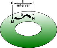
| What we do here is to have a 'function' into this line between the 'equal' objects. This line comes from an interval. |
Paths
In this theory equalities are represented by a path, in a given space.
CTT involves some indirection, so a path is a 'map' from an interval (denoted![]() ) to the proposition that we are proving.
) to the proposition that we are proving.
What happens when there are a sequence of edges following each other? (the target of the first is equal to the source of the second and so on). Can the edge in the interval Is this the same thing as requiring composition? See the page about the graph category for more theory behind this. In cubical type theory equalities are represented by a path, in a given space, between equal terms. |
 |
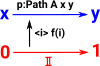
A path can be defined like a function out of the interval p: However, when denoted like that, the endpoints are not visible outside the function (at compile time) so its better to internalise it (with the endpoints as parameters) so the endpoints are visible and denote it like this: PathAx y where:
Although |
 |
Such a path 'type' is a proposition that x and y are equal. We can have such 'types' regardless of whether they are true or false. To prove that this is a true proposition we have to construct an instance of it.
A map out of an interval is not strictly a function, if it was a function it could be constructed with a lambda function like this: p=λi.expression(i) but it is still a binding of the variable 'i' so instead we write it like this: p=<i>expression(i) |
 |
So the Path construct is like a function type but is not strictly a type so we can summarise the different notation as follows:
| Function | Path function out of Interval |
Interval | |
|---|---|---|---|
| formation | A->B | Path A a b | |
| constructor | λ x.exp(x) | p=<i>exp(i) | |
| eliminator | f(x) | p@i |
For more about paths see:
- paths in graph
- paths in simplicial set
- paths in cubical set
Interval
An interval space The interval is like a type, we think of functions from it. Technically it is not exactly a type, for instance, we can't have functions into it. |
0 -> 1 |
| We can have a variable (denoted 'i' here) to range between these two values. | |
| If there are more variables then there are also meets and joins. |
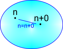
Example n=n+0
| To represent an equality like this we use a path. In the language cubicaltt, when a path is used in a type like Nat directly (heterogeneous path type) it is denoted by PathP. | refl : PathP Nat n n+0 |
For the reasons discussed on this page we instead work more indirectly in terms of a map out of the interval into Nat. This gives a more indirect notion of path denoted by Path in cubicaltt. When we have a function like x->y we interpret this as y for all x. So The n -> at the start shows we want a path that is true for all numbers. So we interpret the whole thing as an equality between the interpretation of n and the interpretation of n+0. |
 |
If we want to prove n=n+0 for all n we want to prove,
but since Nat is infinite we can never do it in this way. However Nat is defined inductively so we can prove this using induction. |
 |
Presheaf
Presheaf Categories
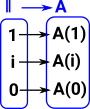
A 'presheaf' category is a special case of a functor category (see page here). It is a contravarient functor from a category 'C' to Set.
Since it is contravarient Cop->Set the homset representing all possible functors can be written:
Hom(Cop,Set)
or
SetCop
There is more about presheaves on the page here.
Cubical sets as presheaf
We can think of this hom functor Cubeop -> set as picking out all cases of a shape (in this case cubes) in set. |
 |
Cubical sets are presheaf categories (quote from site here):
We need cubical because products are closed. This gives 'tiny' interval II in the presheaf category.
For a discussion about the sheaf stucture of simplicial sets see the page here.
Presheaf Example - GraphSee this page. |
 |
Presheaf - Interval
|
 |
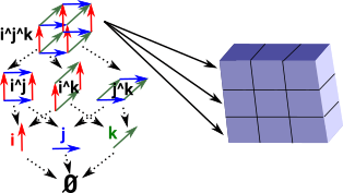
| This diagram tries to relate this to cubical complex bases on combinatorial notation as described on page here. | 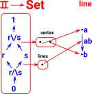 |
| A slightly more complex complex: | 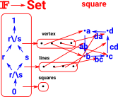 |
Model Category in CTT
We have some nice properties if mappings are continuous. The most general form of continuous map is mapping between topological spaces where all open sets in codomain have preimage which is an open set. However, lines are not open sets in general. To get these properties we need to restrict to structures where we do have these properties such as maps between simplicies.
Fibration in CTT
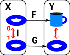
A fibration allows us to 'lift' a line between two points to a line between two structures. This is called the homotopy lifting property (HLP). In this diagram the blue lines show the mapping of points and the green line maps lines (like open set) in the opposite direction to the points. |
 |
Cofibration in CTT
A cofibration allows us to 'extend' a mapping from a subset to a mapping from the whole structure. This is called the homotopy extension property (HEP). Again the blue lines show the mapping of points and the green line maps lines (like open set) in the opposite direction to the points. |
 |
Kan Extensions
The concept of Kan extensions comes from category theory and is introduced on the page here.
We are given 3 categories 'C', 'D' and 'E' and 2 functors F:C->E and K:C->D. The Kan extension tries to find some unique functors between D and E: |
|
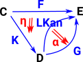
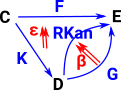
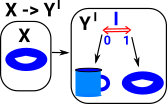
Here we want to use this concept in cubical type theory: So, using the left Kan extension, C becomes the interval, D and E become types we want to compare. |
 |
 |
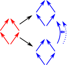
According to this theory it suffices to define this at one end of the interval (say at i=1). The other end of the interval can be inferred. |
We can extend this concept to higher dimensional intervals (for example a square). Provided only one face is missing the orther one can be filled in See fill function on this site. In order to program with these concepts we may need the ability to work with individual arrows (partial functions). Extending one end extends the other. |
 |
Interval Eliminator
The eliminator for functions is function application which is usually indicated by juxtaposition. With a function out of the interval we use '@' to indicate function application. So, if we have a path from x to y we can use this to give us the endpoints.
- p @ 0 = x
- p @ 1 = y
Example from Arend Language The function coe defines dependent eliminator for I, it says that in order to define f : \Pi (i : I) -> P i |
\func coe (P : I -> \Type)
          (a : P left)
          (i : I) : P i \elim i
| left => a |
| From Arend code |
Consequences of Identity Eliminator
From the identity eliminator we can derive equivalence (symmetry, reflexitivity and transitivity) also substitution and unification.
Symmetry of Path
sym (A:U) (a b : A) (p:Path A a b) : Path A b a = <i>p e -1
Reflexitivity of Path
<i>a : Path A a a
a->a
<i>a can be thought of as like λ(i:![]() )->a
)->a
That is constantly a.
Transitivity of Path
For every type A and every x,y,z there is a function:
(x=y) -> (y=z) -> (x=z)
Substitution
Composition
We want to compose two paths:
These correspond to the bottom and right arrows on this diagram: Their composition is the arrow on the top. |
 |
More information on the website here.
Unification
The process of finding a substitution that makes two atomic sentences identical.
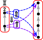
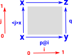
MeetHere we have two variables i and j. We want to look at p at i/\j which is given by: <i,j>p@(i/\j) by substituting 0 and 1 into various combinations of i and j we can get expressions for the edges and points on the diagram: |
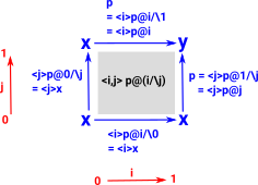 |
JoinIn this case we look at p at i\/j which is given by: <i,j>p@(i\/j) and again we substitute 0 and 1 into various combinations of i and j: |
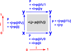 |
Example Bool
For instance in Bool, if we want to prove not(not(x))=x. We don't just have a point not(not(x)) and a point x and a line between them. Instead we have a path as described above.
This path represents a proposition. To prove the proposition we need to construct the type. As this type is a function that is an implementation of the function. |
 |
Example Set
p: Path Set a b is a proposition in set. We can make a proposition of equality between any two elements. <.> x:p is a constructor for this proposition, an implementation of the function out of the interval, so it is a proof of the proposition. In set we can only construct Path Set a a , so this is like Refl for set |
p: Path Set a b <.> x:p |
Paths and Equivalence
Transport turns path into equivalence.
Product Type
Instances of the product type are a tuple. If we require (a,b)=(c,d) then we need a=c and b=d. (eliminator for product type). |
 |
Topological Spaces As Types
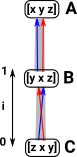
| As discussed on the page here HoTT relates types to spaces: | 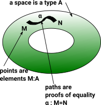 |
| On the page here is a discussion of proofs and how points can be considered equal if they have the same properties. | 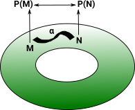 |
There is a problem with modeling spaces in this way in the consistency of higher order equalities. To maintain consistency we need to model in a a less direct way by using the map out of an interval. |
 |
Definition
Every type needs to define
- composition operators: hcomp
- coertion operators: transp
Comparison to Proof in Martin-Löf Theory
On the page here we looked at proofs in a more traditional Martin-Löf theory. When implemented (modeled) in Idris it is shown as an equality which we understand as a proposition. |
(plus x Z) = x |
| To prove that this proposition is true we need to construct it like this: | Refl |
| In order to use cubical type theory as implemented (modeled) in 'cubicaltt' we need some changes. Instead of '=' it uses Path. | Path nat (add zero n) n |
| This path is constructed as a function from the interval like this: | <i> zero |
| So here is a proof in Idris using traditional Martin-Löf theory. | total plusZeroRightNeutral : (x : Nat) -> (plus x Z) = x
plusZeroRightNeutral Z = Refl
plusZeroRightNeutral (S n) = rewrite (plusZeroRightNeutral n)
in Refl |
| Here is the same proof from 'cubicaltt'. Instead of '=' it uses Path. | add_zero : (n : nat) -> Path nat (add zero n) n = split zero -> <i> zero suc n -> <i> suc (add_zero n @ i) |
Where:
So, instead of modeling '=' directly, it is instead modeled indirectly as 'Path'. |
-- Identity types Path (A : U) (a0 a1 : A) : U = PathP (<i> A) a0 a1 refl (A : U) (a : A) : Path A a a =<i> a |
The interval <i> behaves like a type in some ways but not in others. See below for further discusion of the interval where it will be denoted as![]() .
.
The first way of modeling proofs assumes that things can only be equal in one way but here we change this so that things can be equal in multiple different ways. The above example is comparing values so they can only be equal in one way. Below we compare bool to bool, this can be equal to itself in 2 ways:
- where true=true and false=false
- or where true=false and false=true
Here (from this site) the second type of equality is constructed . Transporting true along this equality gives false and false gives true. isoToEquiv : type of A, type of B, A->B,B->A,y->path B,x->path A notK is a proof that not not b = b |
notEquiv : equiv bool bool = (not,isoToEquiv bool bool not not notK notK) |
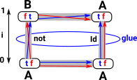
| We can glue these equalities together. | -- Construct an equality in the universe using Glue
notEq : Path U bool bool =
Glue bool [ (i = 0) -> (bool,notEquiv)
, (i = 1) -> (bool,idEquiv bool) ] |
| There are various related mathematical structures that give us multiple perspectives on this. | 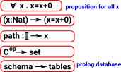 |
Contractible Space
A contractible space is one that can be continuously shrunk to a point within that space.
topological space X is contractible if:
- the identity map on X is null-homotopic,
- if it is homotopic to some constant map.
the following are all equivalent:
- X is contractible (i.e. the identity map is null-homotopic).
- X is homotopy equivalent to a one-point space.
- X deformation retracts onto a point. (However, there exist contractible spaces which do not strongly deformation retract to a point.)
- For any space Y, any two maps f,g: Y -> X are homotopic.
- For any space Y, any map f: Y -> X is null-homotopic.
| (from this site) | -- contractible type isContr (A : U) : U = (x : A) * ((y : A) -> Path A x y) -- The fiber/preimage of a map: fiber (A B : U) (f : A -> B) (y : B) : U = (x : A) * Path B y (f x) -- A map is an equivalence if its fibers are contractible isEquiv (A B : U) (f : A -> B) : U = (y : B) -> isContr (fiber A B f y) |
Variables
| When using 'logic' notation we often specify variables in a context to the left of a 'turnstyle' symbol. |
|
|||
| In programming languages we might specify variables separately somewhere in scope. | Nat n n -> (n = n+0) |
|||
When using cubical type theory we can specify variables in the formal interval: If 'C' is the context, containing the variables, then Cop is the formal interval and a path is a presheaf Cop->Set. |
-- Identity types Path (A : U) (a0 a1 : A) : U = PathP (<i> A) a0 a1 refl (A : U) (a : A) : Path A a a =<i> a |
The Formal Interval
HoTT uses an idea from topology, the interval.
![]() represents the unit interval [0,1]
represents the unit interval [0,1]
not totally ordered like classic interval.
![]() is like a type but it is not a type. Instead a path is a primitive notion in HoTT.
is like a type but it is not a type. Instead a path is a primitive notion in HoTT.
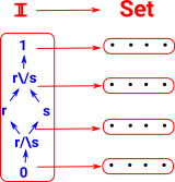
used for variables i... with grammar r,s ::= 0 | 1 | i | 1-r | r/\s | r\/s where:
|
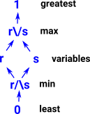 |
Glue
Glue types give us univalance.
Glue types turn an equivalence of types into a path:
ua: (A B : U) -> A ~ B -> PathU A B
Theory
If we have a type B and a partial type A that is equivalent to B where it is defined then we can glue them together to form a new type. |
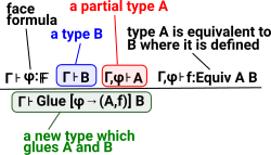 |
Example
Here is an example of a binary type with two elements '0' and '1'. This type can be 'equal' to inself in two ways:
|
 |
So we get two squares that must commute.
Gluing the top mappings together then give one square and the centre of the square can be filled in representing the isomorphism/equality of the whole type with itself.
| Glue type from Agda cubical here | Glue : |
| constructor | glue : |
| eliminator | unglue : |
Where:
|
Partial : |
Partial Types
Composition of Paths and Transport
These may need to be defined for each type. This is done using the glue construct above.
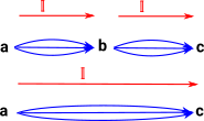
For traditional equalities and equivalences we have a relatively simple concept of transitivity to combine them. So in the case illustrated here:
so we can deduce
|
|
This could be extended to multiple equalities which might be illustrated by a diagram like this where the missing face of a polygon can be inferred. This is related to a Horn clause discussed on page here. |
However, when we move to homotopy type equalities things get more complicated, we need to make sure all possible paths between the endpoints are included. See the discussion of composition of paths on page here. |
 |
Example - List
We have already looks at the 'bool' example. Here is slightly more complicated so that we can think about composition. So imagine a type which is a list containg the elements: 'x', 'y' and 'z'. If we have another list with these elements, but in a different order, then this would be isomorphic (but not equal) to the original list. |
 |
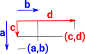
Combining intervals
| Meet | 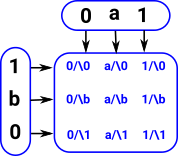 |
| Join | 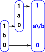 |
Modeling Algebra
| I'm trying to put this all together in one diagram - not correct yet. | 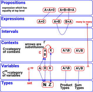 |
Comparison ETT and CTT
| ETT | CTT | |
|---|---|---|
| Introduction | a,b:Nat a=b |
Path Nat a b |
| Construct | Refl : a=b | f:a->b <i>f : Path Nat a b |
| Deconstruct |
Comparison ITT and HoTT
In M-L intentional type theory a proposition is either proven or not, if it was not then it may, or may not, be true. Since proofs in HoTT are canonical then we have other possibilities, it may be true, false, neither or both, also it may be true in many ways. These values represent truth values of propositions which correspond to paths in a space. This situation with different truth values is related to the idea of topos in category theory.
| ITT | HoTT |
|---|---|
Proposition a=b |
Path I->A |
Proof of that proposition Refl: a=a |
λi -> x |
Free De Morgan Algebra
De Morgan algebra is a generalisation of boolean algebra without rule of excluded middle.
RecapSo if we have 2 points 'n' and 'n+0' are they on a path/surface? This corresponds to the proposition 'n=n+0'. If we we using Boolean logic this proposition would be either true or false. In M-L type theory/constructive logic the proposition is either proven or its not, if its not then we can't say anything about it. Here the truth value is a free De Morgan algebra. |
 |
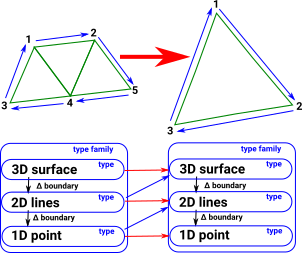
Fibrations
A cubical complex might be thought of as a family of types where the cells are put into are hierarchy of types according to their dimension. These dimensions (and therefore types) are related by their boundary maps, |
 |
Presheaves
Presheaves allow us to build a more complex object out of simpler objects.
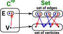
If C is a category of primitive objects then the presheaf is:
F: Cop -> Set
| Objects of C | Morphism in C |
|---|---|
X |
f: X -> Y |
| where: F(X) is a set representing the ways X occurs inside F. |
where: |
| see nlab site | 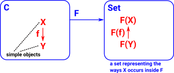 |
Cubical sets are presheaves
Sheaves are discussed on page here.
Kan Composition
More information about Kan composition on these sites:
- https://ncatlab.org/nlab/show/Kan+complex
- https://en.wikipedia.org/wiki/Kan_fibration
- http://www.cse.chalmers.se/~coquand/stockholm.pdf
More information about Kan extensions on page here.
Implementations
| Agda | |
| CubicalTT | |
| Arend | |