On this page we take the topology examples previously introduced on the page here and go on to relate this to the homology of these examples.
First we derive the chain complex.
One Dimensional Facets
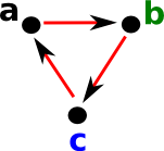
To this example have added designations for the vertices and edges on the diagram on the right:
|
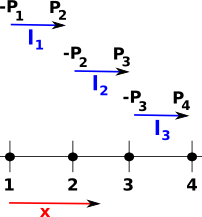 |
This matrix defines the mapping from edges to vertices in this case. In each column of the matrix, representing an edge, We have -1 in the row representing the start of the edge and +1 in the row representing the end of the edge. |
edges |
|||||
| vertices | l1 = [1..2] |
l2 = [2..3] |
l3 = [3..4] |
|||
| P1 | -1 |
0 |
0 |
|||
| P2 | +1 |
-1 |
0 |
|||
| P3 | 0 |
+1 |
-1 |
|||
| P4 | 0 |
0 |
+1 |
|||
In FriCAS we can run as follows: First we setup the cubical complex as described on previous page. |
(1) -> ACUBE := FiniteCubicalComplex(Integer)

   (1)  FiniteCubicalComplex(Integer)
                                     Type: Type
(2) -> vs1:List(Integer) := [1,2,3,4]

   (2)  [1,2,3,4]
                            Type: List(Integer)
(3) -> L1 := cubicalFacet(1,[1..2])

   (3)  (1..2)
                             Type: CubicalFacet
(4) -> L2 := cubicalFacet(1,[2..3])

   (4)  (2..3)
                             Type: CubicalFacet
(5) -> L3 := cubicalFacet(1,[3..4])

   (5)  (3..4)
                             Type: CubicalFacet
(6) -> ln1:=cubicalComplex(vs1,[L1,L2,L3])$ACUBE

   (6)
        (1..2)
        (2..3)
        (3..4)
            Type: FiniteCubicalComplex(Integer)
(7) -> boundary(ln1)

   (7)
        -(1..1)
        (4..4)
Type: FiniteCubicalComplex(Integer) |
We can coerce this into a DeltaComplex which indexes each dimension into the next lower. DeltaComplex is used internally for calculating chain and homology. |
(8) -> d1 := ln1::DeltaComplex(Integer)

   (8)
         1D:[[- 1,2],[- 2,3],[- 3,4]]
             0D:[[0],[0],[0],[0]]
Type: DeltaComplex(Integer) |
| The chain is matrix which goes from edges to to vertices. | (9) -> chain(d1)
+- 1 0 0 +
| | ++
| 1 - 1 0 | ||
(9) [0 0 0 0],| |,||
| 0 1 - 1| ||
| | ++
+ 0 0 1 +
Type: ChainComplex |
| Homology is connected space with no holes. | (10) -> homology(d1)
(10) [Z,0]
Type: List(Homology) |
Another Example
Now we extend this example so that the edges are in a square, but they are still separate edges, we have not yet moved to a solid square.
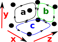
Again I have added designations for the vertices and edges on the diagram on the right:
|
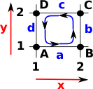 |
| This matrix defines the mapping from edges to vertices. | edges |
||||||
| vertices | a = [1..2,1..1] |
b = [2..2,1..2] |
c = -[1..2,2..2] |
d = -[1..1,1..2] |
|||
| A | -1 |
0 |
0 |
+1 |
|||
| B | +1 |
-1 |
0 |
0 |
|||
| C | 0 |
+1 |
-1 |
0 |
|||
| D | 0 |
0 |
+1 |
-1 |
|||
Again, in each column of the matrix, representing an edge, We have -1 in the row representing the start of the edge and +1 in the row representing the end of the edge. However this time we also have to take into account the sign (orientation) of the edges, reversing +1 and -1 as necessary.
In FriCAS we can run as follows: First we setup the cubical complex as described on previous page. |
(11) -> sps := sphereSurface(2)$CubicalComplexFactory

   (11)
         -(1..1,1..2)
         (2..2,1..2)
         (1..2,1..1)
         -(1..2,2..2)
Type: FiniteCubicalComplex(Integer) |
We can coerce this into a DeltaComplex which indexes each dimension into the next lower. DeltaComplex is used internally for calculating chain and homology. |
(12) -> d2 := sps::DeltaComplex(Integer)

   (12)
          1D:[[1,- 2],[- 1,3],[2,- 4],[- 3,4]]
                  0D:[[0],[0],[0],[0]]
Type: DeltaComplex(Integer) |
| The chain is matrix which goes from edges to to vertices. | (13) -> chain(d2)
+ 1 - 1 0 0 + ++
|- 1 0 1 0 | ||
(13) [0 0 0 0],| |,||
| 0 1 0 - 1| ||
+ 0 0 - 1 1 + ++
Type: ChainComplex |
| Homology is connected space with no holes. | (14) -> homology(sps)
(14) [Z,Z]
Type: List(Homology) |
Two Dimensional Facets
Now we continue with the square example above but this time we treat it as a solid square. The mapping from edge to vertices is the same as above but now we also have a mapping from square to edges.
| In order to represent the homology from this we need to have each mapping indexing into the next. | 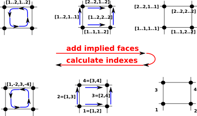 |
So, on the above diagram going across the top row, starting from the square [1..2,1..2] we can generate all possible edges:
and from them we can generate all possible vertices:
Then, going left across the bottom row, we can replace these with indexes so that each dimension indexes into the next. |
(15) -> sp := sphereSolid(2)$CubicalComplexFactory

   (15)
         (1..2,1..2)
            Type: FiniteCubicalComplex(Integer)
(16) -> d5 := sp::DeltaComplex(Integer)

   (16)
                   2D:[[- 1,4,2,- 3]]
          1D:[[- 1,2],[- 1,3],[- 2,4],[- 3,4]]
                  0D:[[0],[0],[0],[0]]
Type: DeltaComplex(Integer) |
Conversion to Chain Complex
Now we have the delta complex we can go on to generate a 'chain complex', this consists of a sequence of matrices which map each array of indices to the next higher array.
I have put a more general discussion of chain complexes on page here.
Once we have added the implied faces we can then give each vertex an index number. The index numbers, for each square, need not be consecutive as in the diagram but:
|
 |
|||||||||||||||||
We can now map to a set of indexes for the edges as follows:
|
|
|||||||||||||||||
| This gives indexes for the edges as shown on the diagram on the right: |  |
|||||||||||||||||
|
||||||||||||||||||
 |
||||||||||||||||||
This matrix defines the mapping Note: the edges are not numbered in the order that we travel around the square, that would be: 1,2,-4,-3. |
square |
|||
| edges | [1..2,1..2] |
|||
| 1 =[1..2,1..1] | +1 |
|||
| 2 =[2..2,1..2] | +1 |
|||
| 3 = -[1..1,1..2] | -1 |
|||
| 4 = -[1..2,2..2] | -1 |
|
(17) -> chain(d5)

                      +- 1  - 1   0    0 + +- 1+
                      | 1    0   - 1   0 | | 1 |
   (17)  [0  0  0  0],|                  |,|   |,[]
                      | 0    1    0   - 1| |- 1|
                      + 0    0    1    1 + + 1 +
                             Type: ChainComplex
(18) -> homology(sp)

   (18)  [Z,0,0]
Type: List(Homology) |
Other Two Dimensional Examples
The above example shows the working for one single square. In a practical two dimensional example we would have multiple squares. To see a page with examples like this, click on these links:
Two Dimensional Facets in Three Dimensional Space
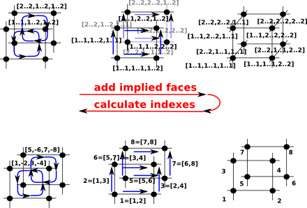
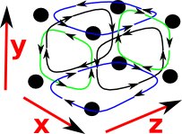
If we continue with two dimensional facets (squares) but now embed them in three dimensional space.
We use the same principle as above, that is, we add the implied faces then we calculate the indexes. As the number of dimensions increases things get a bit more complicated. I tried to put this in one diagram, as above, but this rapidly becomes harder/imposible to draw:
So instead lets look at each stage seperately. Lets look at some faces of a cube (but these are still individual faces, not a solid cube) |
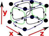 |
Two dimensional faces in 3 dimensions will each have 3 intervals one of which one will be degenerate. So lets look at the boundary of these. For instance:
| δ[1..2,1..2,1]
green cycles on diagram |
(19) -> delta(cubicalFacet(1,[1..2,1..2,1]))

   (19)
   [-(1..1,1..2,1..1),(2..2,1..2,1..1),
   (1..2,1..1,1..1),-(1..2,2..2,1..1)]
Type: List(CubicalFacet) |
| δ[1..2,1,1..2]
blue cycles on diagram |
(20) -> delta(cubicalFacet(1,[1..2,1,1..2]))

   (20)
   [-(1..1,1..1,1..2),(2..2,1..1,1..2),
   (1..2,1..1,1..1),-(1..2,1..1,2..2)]
Type: List(CubicalFacet) |
δ[1,1..2,1..2] black cycles on diagram |
(21) -> delta(cubicalFacet(1,[1,1..2,1..2]))

   (21)
   [-(1..1,1..1,1..2),(1..1,2..2,1..2),
   (1..1,1..2,1..1),-(1..1,1..2,2..2)]
Type: List(CubicalFacet) |
| So a 'square' has two non-degenerate intervals and the direction of rotation around these are given by: |
|
Again, the direction of rotation is given by the left hand rule, but this time the thumb of the left hand is pointing in the direction of the missing dimension then, the fingers curl in the direction of rotation.
on page here.
Once we have added the implied faces we can then give each vertex an index number. The index numbers, for each square, need not be consecutive as in the diagram but:
|
 |
|||||||||||||||||||||||||||||||||||||||||
We can now map to a set of indexes for the edges as follows:
|
|
|||||||||||||||||||||||||||||||||||||||||
| This gives indexes for the edges as shown on the diagram on the right: | 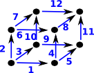 |
|||||||||||||||||||||||||||||||||||||||||
|
||||||||||||||||||||||||||||||||||||||||||
|
||||||||||||||||||||||||||||||||||||||||||
Three Dimensional Facets in Three Dimensional Space
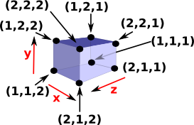
Now we treat the cube as a solid object.
A solid cube in 3D has three dimensions all of which are non-degenerate intervals. So [1..2,1..2,1..2] is a solid cube. |
 |
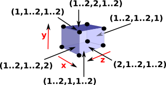
In order to find the boundary of this cube we replace each interval, in turn, with its endpoints. This gives the 6 faces.
The orientation of some of these faces is reversed, this is done in such a way that, if the boundary operator is applied twice, then the edges will cancel out. That is, each edge is common to two faces and each face winds round in such a way that the direction of the common edge cancels out.
This direction is given by the left hand rule: If your left hand thumb points from the inside to the outside of the cube then the fingers curl in the direction of the winding.
When we replace each interval we alternate signs like this: This is familiar from simplicial complexes where we remove each dimension, in turn, and alternate the sign. |
|
In addition to this: the face corresponding to the starting value, in each interval, is reversed and the second value is not.
So both simplicial complexes and cubicial complexes have this structure where we get a boundary by removing each entry in turn and alternating the sign. For simplicial complexes this happens with edges but with cubicial complexes it happens with 2D faces. |
|
| So the boundary of a cube is 6 square faces as expected. | (19) -> sc1 := sphereSolid(3)$CubicalComplexFactory
(19)
(1..2,1..2,1..2)
Type: FiniteCubicalComplex(Integer)
(20) -> sc2 := boundary(sc1)
(20)
-(1..1,1..2,1..2)
(2..2,1..2,1..2)
(1..2,1..1,1..2)
-(1..2,2..2,1..2)
-(1..2,1..2,1..1)
(1..2,1..2,2..2)
Type: FiniteCubicalComplex(Integer) |
| Try delta again, this gives zero and applying the boundary operator twice always gives zero. |
(21) -> sc3 := boundary(sc2)

   (21)  [empty]
            Type: FiniteCubicalComplex(Integer)
|
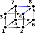
Combinatorics of Cube
We can analyse a cube in pure combinatorics terms, rather than geometric terms, as follows:
| A solid cube represented here as (1..2,1..2,1..2), we can then define subsets of this by making some of the intervals degenerate. | 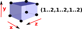 |
From this (1..2,1..2,1..2) cube we can then get the 6 faces by using all possible combinations with one degenerate interval. |
 |
| We can then get the 12 edges by using all possible combinations with two degenerate intervals. | 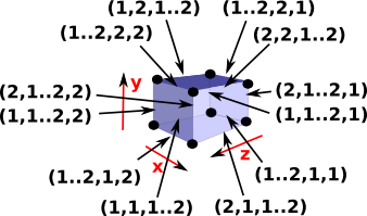 |
We can then get the 8 vertices by using all possible combinations with all three degenerate intervals. |
 |
Orientation of a Face
These n-dimensional faces all have orientations. In order to assign directions to the boundary of a face we need to have a consistent set of conventions, for instance, it would help to always start a the same vertex when going around the boundary.
If we are going from (1,1) to (2,2) on this face it should not matter if we go via (1,2) or (2,1) because it commutes. So, on the diagram, we can go 'a' then 'b' or 'c' then 'd', that is: a + b = c + d which gives: a + b - c - d = 0 |
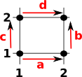 |
So we need to decide which of these to choose as a positive boundary direction. To do this go back to the earlier notation:
Given a face: [1..2,1..2] To generate the boundary δ[1..2,1..2] we start at the minimum vertex [1,1]
|
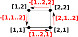 |
So we start at the minimum coordinate indexes, apply the first (non-degenerate) interval, then the second, then minus the first, then minus the second.
The aim of these rules is so that the boundary operator works correctly when the faces are embedded in higher dimensional cubes:
Other Shapes/Spaces
We can construct other common cubical complexes by using CubicalComplexFactory like this: