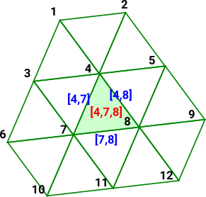
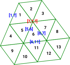
We can label the points, lines, triangles and so on. Each of these dimensions can have its own labeling scheme. Alternatively we could choose a labeling scheme that illustrates the relationship between the dimensions.
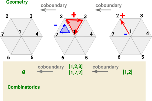
HomologyHomology is point-centric in that we start with the points and the arrows go up to the higher dimensions. So here I have labeled the points by a single index, each line is labeled by a list of the two points it connects, the triangles by 3 indices, and so on. (for now I have not specified the orientation). If there were two lines between the same points then it would be unclear how to uniquely label each line. |
 |
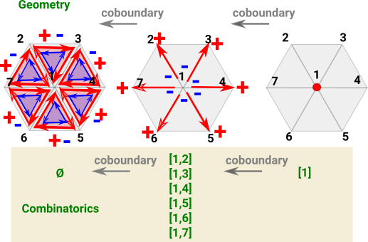
CohomologyCohomology starts with the higher dimensions and the arrows go down to the points. So here I have labeled the triangles with a single index and tried to relate this down the dimensions. The lines have two indices relating a common edge of two triangles, This works on a continuous surface but it is unclear how to label a boundary edge. Also it is unclear how to label points since, in this case, they join 6 triangles but we only need 3 to specify the point. |
 |
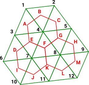
Poincaré DualityPerhaps to get poincaré duality we need to go from triangles to hexagons? |
 |
 |
 |
 |
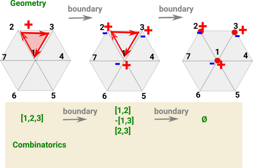
One way to introduce cohomology is to start with homology and reverse the arrows. Can we begin with a chain complex consisting of a sequence of matrices and invert these matrices to get a cochain complex?
There are lots of problems with this:
- The matrices are not all square so to find inverse we have to choose left or right inverse if they exist.
- Matrix inverse involves division by determinant, division may not exist in integers so we would have to go to matrix over rationals.
- Determinant of boundary function tends to be zero, see case below.
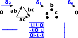
As an example lets use the chain complex of a flat disk: The determinant of this matrix is zero so we can't invert it. |
 |
So the inverse arrows are not just free groups which can be represented by matrices as with homology.
More about reversing the arrows here.
Dual Space
The dual vector space is the set of all s V -> R where
| [ | x1 | ] | |||
| V* =[ a1 a2 a3 ] | V = | | | x2 | | | |
| [ | x3 | ] |
| where a linear functional maps a vector into its underlying real space. This can be shown as a row (covector) times a column (vector): |
|
| If we choose the real value we are mapping to is zero then a vector in a space will map to a plane in its cospace. | 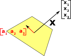 |
Using representable functors
We do this by replacing the free groups by their mapping into set (the integers). This gives a contravariant mapping, see 'representable functor'.
Here we add mappings into the integers Z. Mappings such as these are contravariant |
 |
For instance take disc as example. In order to create a representable functor we create a map which assigns an integer value to each point. This is a map from each point to a scalar value, we can represent this as a co-vector. From this we can derive a map which assigns an integer value to each line and so on, going in the reverse direction. |
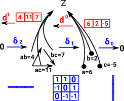 |
| So, for example, the values at each point might represent voltages or heights or somthing like that. | a=6 |
| The lines would then represent voltage differences, or height differences etc. | ab=4 ac=11 bc=7 |
Calculating Cohomology
| So we introduce functions from the elements of the homology (points, lines,triangles ...) to some other quantities. | 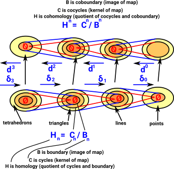 |