 |
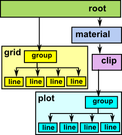
On this page we will create and draw a scenegraph with various plots and a grid in the background. |
Installing the code
Scenegraph graphics has been in FriCAS since FriCAS 1.1.1 but I sometimes update this code so if you need the latest version you can install it as described on this page.
Using the code
Before we can use the scenegraph we need to make the domains available. This is very tedious, it would be better if this was done by default. |
(1) -> )expose SCartesian SCartesian is now explicitly exposed in frame frame1 (1) -> )expose SArgand SArgand is now explicitly exposed in frame frame1 (1) -> )expose SConformal SConformal is now explicitly exposed in frame frame1 (1) -> )expose SceneIFS SceneIFS is now explicitly exposed in frame frame1 (1) -> )expose SceneNamedPoints SceneNamedPoints is now explicitly exposed in frame frame1 (1) -> )expose STransform STransform is now explicitly exposed in frame frame1 (1) -> )expose SBoundary SBoundary is now explicitly exposed in frame frame1 (1) -> )expose ExportXml ExportXml is now explicitly exposed in frame frame1 |
Example 1 - Two dimensional plots with scale.
First we will create a couple of functions to plot:
(1) -> DF ==> DoubleFloat
                                                             Type: Void
(2) -> fnsin(x:DF):DF == sin(x)
   Function declaration fnsin : DoubleFloat -> DoubleFloat has been
      added to workspace.
                                                             Type: Void
(3) -> fntan(x:DF):DF == tan(x)
   Function declaration fntan : DoubleFloat -> DoubleFloat has been
      added to workspace.
                                                             Type: Void
We then need to define what type of algebra to use to define our points, in this case we will use two dimentional Cartesian coordinates:
(4) -> PT ==> SCartesian(2)
                                                             Type: Void
Then we create a bounding box, this is the box within which we do the drawing. For further information about how to use boundaries see page here. This boundary contains two points representing the maximum and minimum extent of the drawing area or volume. That is mins contains the minimum values of x,y… and maxs contains the maximum values of x,y…
(5) -> view := boxBoundary(sipnt(-1,-1)$PT,sipnt(3,1)$PT)$SBoundary(PT)
   (5)  bound box:pt(- 1.0,- 1.0)->pt(3.0,1.0)
                                         Type: SBoundary(SCartesian(2))

(6) -> sc := createSceneRoot(view)$Scene(PT)
   (6)  scene root bound box:pt(- 1.0,- 1.0)->pt(3.0,1.0) #ch=0
                                             Type: Scene(SCartesian(2))

(7) -> gd := addSceneGrid(sc,view)$Scene(PT)
   (7)  scene group #ch=3
                                             Type: Scene(SCartesian(2))
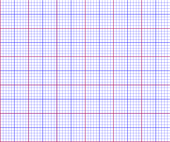 |
We can now export this to a SVG file so that we can confirm that the scene contains a grid: writeSvg(sc,"test1.svg") When we open this file using Inkscape or any other suitable SVG editor then we get the grid on the left. |
We can add axis lines:
(8) -> addSceneRuler_
	   (sc,"HORIZONTAL"::Symbol,spnt(0::DF,-0.1::DF)$PT,view)$Scene(PT)
   (8)  scene group #ch=21
                                             Type: Scene(SCartesian(2))

(9) -> addSceneRuler_
         (sc,"VERTICAL"::Symbol,spnt(-0.1::DF,0::DF)$PT,view)$Scene(PT)
   (9)  scene group #ch=21
Type: Scene(SCartesian(2)) |
Now lets add a plot to this. First we add a 'material' node to the root to define the colour and thickness of the plot. Then we add the plot to the material node using the sine function that we defined earlier.
(10) -> mt1 := addSceneMaterial(sc,3::DF,"blue","green")$Scene(PT)
   (10)  scene material lw=3.0 lc="blue" fc="green" mo=1.0 #ch=0
                                             Type: Scene(SCartesian(2))

(11) -> ln1 := addPlot1Din2D(mt1,fnsin,0..3::DF,49)$Scene(PT)
   Compiling function fnsin with type DoubleFloat -> DoubleFloat
   (11)  scene line [[pt(0.0,0.0),pt(0.0625,0.0624593178423802),....]] #ch=0
                                            Type: Scene(SCartesian(2))
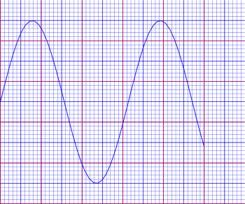 |
We can now export this to a SVG file again to see that the plot has been added to the grid: writeSvg(sc,"test2.svg") Again we can open this file using Inkscape to see the results. |
Lets now add second plot to the scene so that we can see how to modify it using material and clip. If we did not clip the tangent function it would extend outside of our drawing area and we would also get a vertical line at the singularity at pi where the value jumps from plus infinity to minus infinity. We therfore create a boundary bb at line 13 and clip to that boundary at line 14. This clip node affects all nodes under it.
(12) -> mt2 := addSceneMaterial(sc,3::DF,"green","green")$Scene(PT)
   (12)  scene material lw=3.0 lc="green" fc="green" mo=1.0 #ch=0
                                             Type: Scene(SCartesian(2))

(13) -> bb := boxBoundary(sipnt(0,-1)$PT,sipnt(3,1)$PT)$SBoundary(PT)
   (13)  bound box:pt(0.0,- 1.0)->pt(3.0,1.0)
                                         Type: SBoundary(SCartesian(2))

(14) -> bb2 := addSceneClip(mt2,bb)$Scene(PT)
   (14)  scene clip bound box:pt(0.0,- 1.0)->pt(3.0,1.0) #ch=0
                                             Type: Scene(SCartesian(2))

(15) -> ln2 := addPlot1Din2D(bb2,fntan,0..3::DF,49)$Scene(PT)
   Compiling function fntan with type DoubleFloat -> DoubleFloat
   (15)  scene line [[pt(0.0,0.0),_
                           pt(0.0625,0.06258150756627502),....]] #ch=0
                                             Type: Scene(SCartesian(2))

(16) -> addSceneText(sc,"sin(theta)",32::NNI,_
                   spnt(0.5::DF,0.4::DF)$PT)$Scene(PT)
   (16)  scene text="sin(theta)" sz=32 p=pt(0.5,0.4) npt=[] #ch=0
                                             Type: Scene(SCartesian(2))

(17) -> addSceneText(sc,"tan(theta)",32::NNI,_
                   spnt(0.1::DF,0.6::DF)$PT)$Scene(PT)
   (17)  scene text="tan(theta)" sz=32 p=pt(0.1,0.6) npt=[] #ch=0
                                             Type: Scene(SCartesian(2))
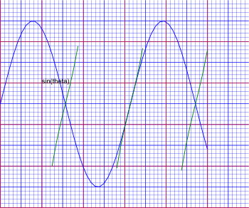 |
We can now export this to a SVG file to see the combined result: writeSvg(sc,"test3.svg") Again we can open this file using Inkscape to see the results. |
Next Stage
For a tutorial about how to transform these shapes see this page.
Further Information
Other aspects of the graphics framework on these pages:
- User Reference on this page.
- Programmers Reference on this page.
- Examples of scenegraph structure on this page.
- The code is in file: scene.spad.pamphlet which is available from here.
- Existing Axiom graphics framework on this page.