Summary
When we are working in a two dimensional plane we can represent angular velocity by a single number. In three dimensions we can represent angular velocity as a three dimensional vector quantity (wx, wy, wz). In this form angular velocities can be combined using vector addition.
This is in contrast to finite rotations (as explained on this page) which need extra dimensions in order to avoid singularities and to correctly combine finite rotations.
Two Dimensional Case
With linear movement things are relatively simple, we just use v = dx/dt, velocity 'v' is the rate of change of distance with time, we treat it as being the same thing as dx/dt
If we are working in two dimensions then we can define angular velocity 'w' in a similar way:
w = d angle/dt
In other words, if we are measuring the angular velocity of a moving point, it is the rate of change of the angle it makes compared to some reference direction. Of course this will depend on the point we are measuring the angle from. In some cases this is easily implied, for example if we are measuring the angular velocity of a solid object rotating about its centre of mass, then we would usually measure the angle of some point relative to the centre of mass. However its not always obvious where we are measuring from so we should be careful to define it.
Body rates ( )
)
For a three dimensional solid body these are the rotational rates that could be measured by rate gyros with their sensing axes aligned with the appropriate body coordinate axes; they also can be calculated from the dynamic equations of motion.
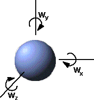
The angular velocity can be specified by a 3D vector:
| wx |
| wy |
| wz |
The components of this vector represent vector sum of:
- wx: the rate of change of angle (in radians) about the absolute x coordinate.
- wy: the rate of change of angle (in radians) about the absolute y coordinate.
- wz: the rate of change of angle (in radians) about the absolute z coordinate.
wx,wy and wz are independent of each other, so angular velocities can be added, if appropriate, without any of the issues involved with euler angles. This is because we are adding infinitely small angles which have the same properties as vectors. See this example which involves adding angular velocities.
Euler rates
Euler rates are what we get when we differentiate Euler angles, for example:
d heading / d t
d attitude / d t
d bank / d t
At first sight it may appear that Euler rates are the same as body rates described above, this is not the case however. If a solid object is rotating at a constant rate then its body rate (wx, wy, wz) will be constant, however the Euler rates will be varying all the time depending on some trig function of the instantaneous angle between the body and absolute coordinates. So Euler rates are very messy, they have singularities and they are not of much practical use.
So the main reason for mentioning Euler rates here is to make the distinction with body rates and to warn people to avoid use of Euler rates.
Representing Angular Velocity using Axis-Angle
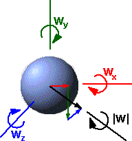
See this page for axis-angle notation for finite rotations.
Imagine a solid object which has simultaneous rotation about the x,y and z axes, the angular velocity about these axes is wx,wy and wz. This rotation could also be represented by a single rotation about the axis (wx, wy, wz).
- angular speed = d angle/d t = |w(t)| = √(wx2+wy2+wz2).
- normalised axis =(wx,wy,wz)/ |w(t)|
| where: | |||
symbol |
description |
type |
units |
| ω | angular velocity | bivector | s-1 |
| angle | angle in radians | scalar | none |
| t | time | scalar | s |
| d ... /dt | rate of change | ||
Axis angle is only applicable for continuous rotations like this when rotation is only around the axis, in this case rotation is in one plane and this is equivalent to the 2D case, in other words the axis represents the 2D plane we are operating in.
We can't really use axis angle to combine angular velocities in different directions.
Differentiating Rotation Matrices and Quaternions
When we are working in terms of matrices or quaternions the equation is more complicated:
- for matrices it is: [d R(t) / dt] = [~w]*[R(t)]
- for quaternions it is: d q(t) /dt = ½ * W(t) q(t)
These equations are proved and defined further down this page.
What are the deeper reasons for this extra complexity. I think this involves these factors:
- These are time varying quantities, of course v = dx/dt also works for time varying quantities, but at least if we have constant velocity (and so constant linear momentum) then dx/dt will be constant. But if [R(t)] represents the orientation of an object rotating at a constant angular velocity (and constant angular momentum) then [d R(t) / dt] will still vary with time but [~w] and W(t) , as used in the above equations, will not vary with time and therefore are a better representation of angular velocity.
- Differentiation is related to the addition operation, but rotations are combined using matrix multiplication, not addition. When I say "differentiation is related to the addition operation" I mean: when we add a small increment to time we get a small increment to distance, differentiation is the limit when these additions. So is there a mathematical theory that relates small incremental multiplications to conventional differentiation?
Even if we are using matrices or quaternions to represent 3D orientations and rotations, when we translate these to angular velocities, we will probably want to express these as 3D vectors. The values W(t) and [~w] in the above equations can easily be converted to 3D vectors, W(t) is virtually a 3D vector already and the skew symmetric matrix [~w] has all the elements of the 3D vector.
The reason for expressing angular velocities in terms of 3D vectors is that it is often valid to combine angular velocities by adding their 3D vectors. So the properties of angular velocities are completely different from the properties of finite rotations.
Angular Velocity of Particle
Here we derive the rotation values from a point mass (particle). The point mass is not necessarily rotating about its own axis (although it could, subatomic particles have spin). What we are interested in here is the contribution of the particle to the rotational properties of a bigger mass about some fixed point. For further explanation try reading numerical methods.
Consider a point mass at ![]() .
Its linear velocity is the cross product of its angular velocity about
.
Its linear velocity is the cross product of its angular velocity about ![]() and its distance from
and its distance from ![]() .
.
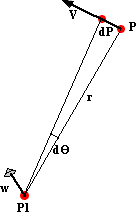
dP = r dθ
So differentiating both sides with respect to time and representing in vector
notation with ![]() perpendicular to both
perpendicular to both ![]() and
and ![]() (
(![]() is out of screen/paper toward viewer, note we are using a right
hand coordinate system and a right
hand rule for positive rotation direction)
is out of screen/paper toward viewer, note we are using a right
hand coordinate system and a right
hand rule for positive rotation direction)
![]() =
= ![]() ×
×![]()
| where: | |||
symbol |
description |
type |
units |
| instantaneous linear velocity of particle | vector | m/s | |
| instantaneous angular velocity about |
bivector | s-1 | |
| instantaneous position of the particle relative to point. |
vector | m | |
| × | vector cross product operator (see here for definition) | ||
So the rotation velocity of a point is not an absolute value, but it depends
on which point that the rotation is measured about. Also the particle does not
have to be traveling in a circle to have an angular velocity, it can have a
non-zero angular velocity about ![]() ,
even if the particle is traveling in a straight line, provided
,
even if the particle is traveling in a straight line, provided ![]() is not on the line.
is not on the line.
Angular Velocity of solid object()
The following pages will then go on to derive quantities for finite solid bodies by integrating across the volume. Most of these quantities are vectors of dimension 3 which has a component in the x,y and z directions. To denote a vector quantity we show an arrow above the quantity, for more information about vectors see here.
Consider a point mass at ![]() .
Its linear velocity is the cross product of its angular velocity about
.
Its linear velocity is the cross product of its angular velocity about ![]() and its distance from
and its distance from ![]() .
.
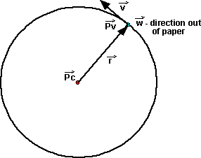
As seen in the Angular Velocity of particle section, angular velocity depends on the point that we are measuring the rotation about. So for a solid object, the angular velocity of all the particles, from which it is composed, are different.
Only when we are measuring the rotation about the centre of rotation is the rotation of all points on the object the same. So, for that reason, when we are talking about the angular velocity of a solid object we mean the angular velocity about its centre of rotation.
If an object is moving in free space, with no external forces or torques acting on it, then it will rotate about its centre-of-mass. So we can represent the total instantaneous motion of a rigid body by a combination of the linear velocity of its centre of mass and its rotation about its centre of mass.
The angular velocity vector W(t) can be derived from the angular position, as a function of time, using various notations:
| in 2D (or 3D with fixed axis) | W(t) = d theta /dt |
| in 3D using matrix | [~w] = [ d T(t) / dt] [T(t)]-1 |
| in 3D using quaternion | W(t) = 2 *d q(t) /dt*conj(q(t)) |
These expressions are derived later in this page.
In the pages about kinematics the position of an unconstrained rigid body was represented by 6 dimensional vector as follows:
| wx | angular velocity the about x axis (radians per second) |
| wy | angular velocity the about y axis (radians per second) |
| wz | angular velocity the about z axis (radians per second) |
| vx | linear velocity of centre of mass along x axis (metres per second) |
| vy | linear velocity of centre of mass along y axis (metres per second) |
| vz | linear velocity of centre of mass along z axis (metres per second) |
Further information about angular velocity.
Representing angular velocity using matricies
For information about differentiating a matrix see this page.
We have already seen that a 3D vector is sufficient to hold all the necessary information about angular velocity. However there may be situations where we might want to hold this information in a matrix. In that case we can use the following matrix:
| [~w]= |
|
This angular velocity matrix is related to the differential of the rotation matrix as follows:
[~w] = [ d T(t) / dt] [T(t)]-1
Mark Ioffe has kindly sent me a derivation which I have adapted to use the notation used on this site.
Let X(t) represent any point on a rigid body as a vector from the origin and let:
X(t) = [T(t)] X(0)
| where: | |||
symbol |
description |
type |
units |
| X(t) | any point on a rigid body at time 't' as a vector from the origin | vector | m |
| [T(t)] | rotation (orthogonal) which transforms vectors at t=0 to vectors at t | matrix | none |
| X(0) | the same point at time 't=0' as a vector from the origin | vector | m |
differentiating this equation gives the linear velocity of the point on the rigid body:
v(t) = d X(t) / dt = [ d T(t) / dt] X(0)
since X(0) is not a function of time.
Inverting the first equation gives:
X(0) = [T(t)]-1 X(t)
so combining these gives:
v(t) = [ d T(t) / dt] [T(t)]-1 X(t)
We know, from the top of this page that, v(t) = w × X(t)
| where: | |||
symbol |
description |
type |
units |
| v(t) | linear velocity vector of given particle | vector | m/s |
| ω | angular velocity vector | bivector | s-1 |
| × | vector cross product | ||
| X(t) | position of given particle | vector | m |
We can convert this cross product expression into an equivalent matrix expression by replacing the w vector by an equivalent matrix [~w] known as a skew-symetric or anti-symetric matrix. which is related to the ω vector as follows:
| [~ω]= |
|
Combining these expressions for v(t) gives:
[~w] X(t) = [ d T(t) / dt] [T(t)]-1 X(t)
removing the X(t) from both sides makes this into a matrix expression for w:
[~w] = [ d T(t) / dt] [T(t)]-1
For more information about this see here.
Representing angular velocity using quaternions
For information about differentiating a quaternion see this page.
If an object is rotating then the quaternion representing its orientation will be a function of time, we therefore denote it by q(t). The differentiation of this is given by:
d q(t) /dt = 1/2 * W(t) q(t)
| where: | |||
symbol |
description |
type |
units |
| q(t) | normalised quaternion representing orientation as a function of time | quaternion | |
| W(t) | angular velocity vector represented as quaternion with zero scalar part, i.e W (t ) = (0, W x (t ), W y (t ), W z (t )) |
bivector | s-1 |
| t | time | scalar | s |
The derivation of this was kindly sent to me by Mark Ioffe here: pdf file
This is expanded out using quaternion multiplication rule:
d q0(t) / dt = − 1/2* (Wx (t) q1(t) + Wy (t) q2(t) + Wz (t) q3(t))
d q1(t) / dt = 1/2* (Wx (t) q0(t) + Wy (t) q3(t) − Wz (t) q2(t))
d q2(t) / dt = 1/2* (Wy (t) q0(t) + Wz (t) q1(t) − Wx (t) q3(t))
d q3(t) / dt = 1/2* (Wz (t) q0(t) + Wx (t) q2(t) − Wy (t) q1(t))
ExampleImagine an object rotating at a constant rate of w radians per second about the z axis. From this page we know that: q = cos(a/2) + i ( x * sin(a/2)) + j (y * sin(a/2)) + k ( z * sin(a/2)) where:
So, in this case, a=w*t and x,y,z=0,0,1 so, q(t) = cos(wt/2) + k sin(wt/2) and, W(t) = k w therefore, d q(t) /dt = 1/2 * W(t) q(t) = 1/2 * k*w*(cos(wt/2) + k sin(wt/2)) = 1/2 * w*(-sin(wt/2) + k cos(wt/2)) |
What I really want to do is show an easy way to swap between using quaternions for representing orientations and vectors for representing angular velocity. I think this does that, but it would be clearer to reverse the example, ie,
q(t) = cos(wt/2) + k sin(wt/2)
derive d q(t) /dt = 1/2 * w*(-sin(wt/2) + k cos(wt/2)) just by differentiating the terms in the above equation.
then derive W(t) = k w from d q(t) /dt = 1/2 * W(t) q(t)
This shows that by differentiating a quaternion we get a vector.
my previous attempt at working this out
Angular Velocity in terms of Euler Angle Rates
The angular velocity vector in body coordinates is:
Wx = rollrate - yawrate * sin(pitch)
Wy = pitchrate * cos(roll) + yawrate * sin(roll) * cos(pitch)
Wz = yawrate * cos(roll) * cos(pitch) - pitchrate * sin(roll)
Jenny has kindly sent me a derivation of this in this document: pdrderivation.pdf.
Using Vector Calculus to analyse rotation of solid objects
Vector Calculus is often used to analyse the movement of fluids, but there is no reason why we should not use it to analyse solid objects, provided that we apply it to regions of space where the vector field is continuous..
If we take a velocity field of a rotating object we might get a field that looks like this:
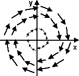
If we take the curl of this field we would get a different vector field
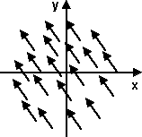
Each of these vectors has the value w2 into the line along the axis of rotation (as proved here)
Representing Angular Velocity in program
Angular velocity in 3D space can be held in a quaternion (see class sfrotation) or a matrix (see class sftransform). For an example of how this might be used in a scenegraph node, see here.


