This page introduces the subject of transformations and links on to other pages which analyse the various types of transform in more detail.
A transform maps every point in space to a (possibly) different point.
There are lots of ways to categorise transforms, one way is to start with the simple transforms that we intuitively understand like:
We can combine these in various ways: combinations of translation and rotation, known as isometries, are important because they represent the ways that solid objects can move in the world without changing shape.
We can also categorise by the types of algebra that can produce the transform, for example, linear (matrix) algebra.
Also we can do transforms in different numbers of dimensions.
Here is an (incomplete) attempt to categorise these things:
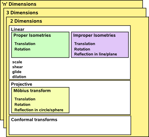
Its hard to categorise these things in a definitive way, for example, projective transforms can be considered linear if we use homogeneous coordinates.
There are different algebras that can represent transforms and help us calculate the effect of different operations, such as combining two transforms, not all of these algebras can represent all transforms. Useful algebras include:
There are two types of algebra associated with transformations (such as rotation) and these algebras must interwork correctly together.
- The first type of algebra defines how a given point is transformed, that is, a given rotation must define where every point, before the rotation, ends up after the rotation.
- The second type of algebra defines how rotations can be combined, that is, we first do 'rotation 1' then we do 'rotation 2' this must be equivalent to some combined rotation, say: 'rotation 3'.
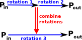 |
The diagram on the left tries to illustrate this.
|
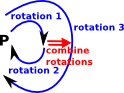 |
Even the above diagram does not fully capture the whole situation because we can apply many transforms, one after the other. What we have is a set of points in a space and maps from this space to itself. On the left I have tried to redraw the above diagram, but looped back to itself. However drawing it in this way starts to get too cluttered. |
One way to try to understand these things is to look at concepts from a branch of mathematics called 'category theory'. this is probably the most abstract way to approach this topic. For 'abstract' read hard but very powerful. Unless you know abstract mathematics (or program in Haskell) you may not know category theory, more about it here.
Isomorphism
We need to have an equivalence between our algebra and the physical transforms, this equivalence is known as an isomorphism (discussed on this page).
Group: set of all quaternions with multiplication |
Group: set of all orientations of a solid object in 3D space with operation composition |
 |
|
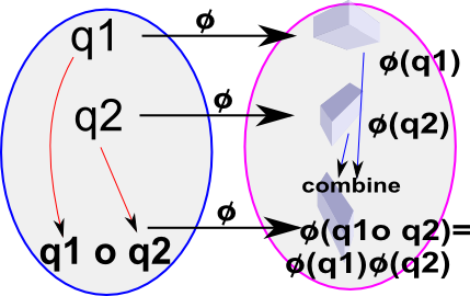
We need an operation, denoted by 'o' here, which represents composition of rotation. The mapping between elements in the algebra and the physical position of the object is represented by 'φ'. We need this to give the same result regardless of whether we do the composition first or the mapping to the real world first, which means,
φ(v1) o φ(v2) = φ(v1 o v2)
where:
- φ = isomorphism mapping
- v1 and v2 = elements of group
- o = group operation
If the group operation 'o' is vector addition '+' then the isomorphism relationship will hold if for the mapping φ(v) we use scalar multiplication m*v which gives:
m*v1 + m*v2 = m*(v1 + v2)
This is known as a vector space and it can be used to represent translations in space.
If the group operation 'o' is quaternion multiplication '*' then the isomorphism relationship will hold if for the mapping φ(v) we use the 'sandwich product' : φ(v) = q v q-1 so
| φ(q1*q2) = q q1 q2 q-1 = q q1 q-1 q q2 q-1 = φ(q1)*φ(q2) |
(since q-1 q =1) |
This 'sandwich product' occurs in many algebras with multiplication such as quaternions, clifford algebra and so on and can represent transforms such as rotations. In the general case this can be thought of as multiplication of vector spaces.
If we try this approach with matrix multiplication we get:
[M][v1] * [M][v2] = [M][v1 * v2]
Which requires the definition of the multiplication of two vectors, if we take the dot product we have:
[M][v1] • [M][v2] = [M][v1 • v2]
So if we take v1 and v2 as being orthogonal to each other, say vx and vy then,
[M][vx] • [M][vy] = [M][vx• vy] = 0
So we need a matrix [M] that, if vectors are orthogonal, then the matrix [M] will maintain that orthogonality. A rotation matrix is such a matrix.
Linear Transforms
Calculations on linear transforms can be done most conveniently using vectors and matrices like this:
|
= |
|
|
The details of how to calculate these transforms are shown on this page.
If we want to include translations then we can use vector addition as follows:
|
= |
|
|
+ |
|
Or, alternatively, we can avoid addition (which makes it easier to combine successive transforms) by increasing the dimension of the vectors and matrices like this:
|
= |
|
|
We can work in higher dimensions by increasing the dimension of the vectors and matrices.
If we want to restrict ourselves to rotations and translations (perhaps occasionally scaling) then we may find other types of algebra more convenient. For instance, to represent a two dimensional rotation and translation, we might use:
v_out = v_in0 * rotation + translation
where these quantities are all complex numbers.
Again we can remove the need for addition by increasing the dimension of our mathematical element, in this case we could use dualComplex numbers.
Again we can work in a higher number of dimensions (say 3D) by using quaternions or dual quaternions. In that case the form of the equations changes to use the 'sandwich form' as described on these pages.
We can completely generalise this to 'n' dimensions by using an even subset of Clifford Algebra.
Projective Transforms
This extends the possible types of transforms to include things like reflection in a circle or sphere. It is an important subject because its used when we are representing a 3D world on a 2D plane in a way that it appears to our eye. For instance: horizontal lines appear to meet at the horizon. For an application of this see OpenGL pages.
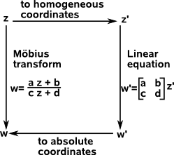
Projective transforms and the Möbius transform are also important in physics, for instance, Roger Penrose uses the stereographic projection to analyse relativity.
Although projective transforms are not, in general, linear (they are a superset of linear transforms) they can be specified in a linear like form (matrix whose elements are complex numbers) by converting to homogeneous coordinates.
More information about projective transforms on this page.
Transform Parameters
There are a number of quantities associated with each transform including the following:
Determinants
This tends to be associated, in peoples minds, with matrices. In fact it can have a geometric meaning which can be calculated from other types of algebras.
It is a scalar value and it is related to:
- The scaling factor of the transform
- The left or right handedness of the transform.
In other words does it make an object bigger or smaller and does it reflect it (an odd number of times).
The calculation of determinants, in the case of matrices, is shown on these pages.
Eigenvalues and Eigenvectors
This also tends to be associated, in peoples minds, with matrices. Again these quantities can have a geometric meaning which can be calculated from other types of algebras.
This tells us something about the symmetry of a transform.
An eigenvector is a vector whose direction is not changed by the transform, it may be stretched, but it still points in the same direction.
Each eigenvector has a corresponding eigenvalue which gives the scaling factor by which the transform scales the eigenvector. So the eigenvector is a vector and the eigenvalue is a scalar.
A given transform may have more than one eigenvector and eigenvalue pair depending on how many dimensions we are working in. For instance:
- If we are working in 2 dimensions there are upto 2 eigenvector and eigenvalue pairs.
- If we are working in 3 dimensions there are upto 3 eigenvector and eigenvalue pairs.
and so on.
The calculation of eigenvectors and eigenvalues, in the case of matrices, is shown on these pages.
As an example, if we have a rotation transform in 3 dimensions, then the eigenvector would be the axis of rotation since this is not altered by the transform and the corresponding eigenvalue would be +1 since the axis is not scaled by the rotation. If we have a rotation in 2 dimensions then the eigenvectors would be ±i where i is √-1 since all vectors in the plane change direction.
Another geometrical application of eigenvectors and eigenvalues is to attempt to factor transforms into rotational and scaling parts, this is discussed on this page.
A more physical application is to the inertia tensor where the eigenvectors indicate the axies that the solid object will rotate around without wobble.
Next
An important class of transforms are rotations and so we can go on to look at these in more detail on these pages.