As an alternative to simplicial complexes, implemented here, we can base our topology on squares rather than triangles. I have tried to base this cubical complex code on the Computational Homology book (see box below). Books written for humans can leave some details of orientations and so on to the reader, but computer code needs to specify the details consistently so I have tried to make these choices explicit on this page.
| Comparison with simplicial complex: |
|
However we need to implement this in a different way, if we specified a square by its vertices then we could not be sure that the vertices were all in the same plane and we could not be sure that the squares aligned.
We therefore have separate indexes for each dimension and we specify these as an interval.
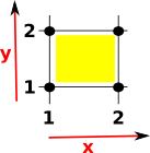
So if we wanted to specify a square with 'x' dimension having an interval from 1 to 2 and the 'y' dimension having an interval from 1 to 2, we would specify it like this:
Square
(1) -> SQUARE := cubicalFacet(1,[1..2,1..2])

   (1)  (1..2,1..2)
Type: CubicalFacet |
 |
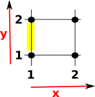
If we want to specify a shape in a higher dimension than the shape itself then some of the intervals will be degenerate, that is, the start and end indexes will be the same. So, for instance, we could specify a line in a 2 dimensional space like this:
Line
(2) -> LINE := cubicalFacet(1,[1..1,1..2])

   (2)  (1..1,1..2)
                               Type: CubicalFacet
|
 |
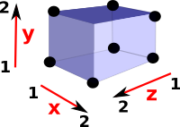
We go to higher dimensions by specifying more intervals like this:
Cube
(3) -> CUBE := cubicalFacet(1,[1..2,1..2,1..2])

   (3)  (1..2,1..2,1..2)
                               Type: CubicalFacet
|
 |
FriCAS implementation of Domains
The structures on this page are encoded in the CubicalFacet and FiniteCubicalComplex domains.
CubicalFacet holds individual facets. Its representation is as follows:
Rep := Record(mul:Integer,fac:List(Segment(Integer)))
- 'fac' is a list of intervals.
- 'mul' encodes the orientation. When we are interpreting this as a geometric object it is usually 1 or -1 (to reverse direction). When we are interpreting this as a linear algebra object then we treat it as an integer.
In the Computational Homology book (see box below right) this is called an Elementary Cell, the elementary cell only allows each interval to be either: l..l or l..(l+1) however this restriction is not enforced in the representation or the code. I think it may be acceptable to allow a CubicalFacet to have a wider range, say l..(l+2), provided we are very clear that this represents multiple Elementary Cells, in this case l..(l+1) and (l+1)..(l+2).
FiniteCubicalComplex holds multiple factets. They can all be different dimensions but they should all have the same number of intervals. If the number of dimensions is less than the number of intervals then, some of those intervals will be degenerate.
Its representation is as follows:
Rep := Record(VERTSET:VS,CUBE:List(CubicalFacet))
Representation holds whole Cubical Complex. This consists of a vertex set, here represented as a vertex list so that we can index it. Also a list of hypercubes.
Vertex Coordinates
In the Computational Homology book potential applications are described such as analyzing images and 3D scans where the elements are pixels or their higher dimensional counterparts. For this type of application we don't really need to define absolute coordinates we can just think of it as an abstract array, so for most purposes we can work with types like this:
FiniteCubicalComplex(VertexSetAbstract)
It is very hard to think why we would ever need to specify coordinates but I would still like to have the possibility to do so for the following reasons:
- To keep the structure as general and adaptable to unforeseen applications as possible.
- To keep compatibility with simplicial complexes where concrete geometries are useful.
If we do work in geometric terms and if we specify vertices as vectors then it is important to note the differences from simplicial complexes.
 |
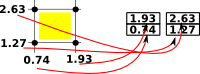 |
| In the case of a simplicial complex we can encode a square as two triangles and each of its vertices can index into a table of vectors. | In the case of a cubical complex the indexes are separate and therefore the coordinates are not held as vectors. |
Therefore the vertex set needs to hold a real (floating point) value for each index in each dimension.
One Dimensional Facets
Line segments (AKA edges) have a direction and we need to make an arbitrary decision about which direction is positive. Here I chose to make the line go from a negative point to a positive point.
(4) -> ACUBE := FiniteCubicalComplex(Integer)

   (4)  FiniteCubicalComplex(Integer)
                                     Type: Type
(5) -> vs1:List(Integer) := [1,2,3,4]

   (5)  [1,2,3,4]
                            Type: List(Integer)
(6) -> L1 := cubicalFacet(1,[1..2])

   (6)  (1..2)
                             Type: CubicalFacet
(7) -> L2 := cubicalFacet(1,[2..3])

   (7)  (2..3)
                             Type: CubicalFacet
(8) -> L3 := cubicalFacet(1,[3..4])

   (8)  (3..4)
                             Type: CubicalFacet
(9) -> ln1:=cubicalComplex(vs1,[L1,L2,L3])$ACUBE

   (9)
        (1..2)
        (2..3)
        (3..4)
            Type: FiniteCubicalComplex(Integer)
(10) -> boundary(ln1)

   (10)
         -(1..1)
         (4..4)
Type: FiniteCubicalComplex(Integer) |
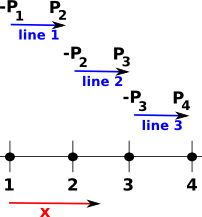
When we take the boundary of these three lines we get -P1 and P4 so because the starting boundary is taken as negative and the finishing boundary as positive the intermediate points cancel out. |
Two Dimensional Facets
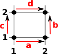
In the same way the edges have an orientation so do two dimensional facets (AKA squares). This orientation is a direction of rotation around the square, I have taken a positive rotation as being:
|
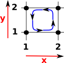 |
This direction of rotation is given by the left hand rule, which is: if the thumb of your left hand is pointing into the diagram then, the fingers curl in the direction of rotation.
(11) -> Sq1 := cubicalFacet(1,[1..2,1..2])

   (11)  (1..2,1..2)
                             Type: CubicalFacet
(12) -> Sq2 := cubicalFacet(1,[2..3,1..2])

   (12)  (2..3,1..2)
                              Type: CubicalFacet
(13) -> Sq3 := cubicalFacet(1,[3..4,1..2])

   (13)  (3..4,1..2)
                               Type: CubicalFacet
(14) -> ex1:=cubicalComplex(vs1,[Sq1,Sq2,Sq3])$ACUBE

   (14)
         (1..2,1..2)
         (2..3,1..2)
         (3..4,1..2)
            Type: FiniteCubicalComplex(Integer)
(15) -> boundary(ex1)

   (15)
         -(1..1,1..2)
         (1..2,1..1)
         -(1..2,2..2)
         (2..3,1..1)
         -(2..3,2..2)
         (4..4,1..2)
         (3..4,1..1)
         -(3..4,2..2)
Type: FiniteCubicalComplex(Integer) |
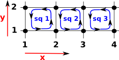
Similar to the lines above, when we take the boundary operator of these three squares the adjacent lines cancel out and we get a rectangle going around the outside. |
Two Dimensional Facets in Three Dimensional Space
If we continue with two dimensional facets (squares) but now embed them in three dimensional space things get a bit more complicated. Lets look at some faces of a cube (but these are still individual faces, not a solid cube) |
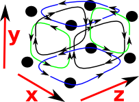 |
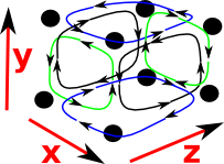
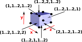
Two dimensional faces in 3 dimensions will each have 3 intervals one of which one will be degenerate. So lets look at the boundary of these. For instance:
| δ[1..2,1..2,1]
green cycles on diagram |
(16) -> boundary(cubicalFacet(1,[1..2,1..2,1]))

   (16)
   [-(1..1,1..2,1..1),(2..2,1..2,1..1),
   (1..2,1..1,1..1),-(1..2,2..2,1..1)]
Type: List(CubicalFacet) |
| δ[1..2,1,1..2]
blue cycles on diagram |
(17) -> boundary(cubicalFacet(1,[1..2,1,1..2]))

   (17)
   [-(1..1,1..1,1..2),(2..2,1..1,1..2),
   (1..2,1..1,1..1),-(1..2,1..1,2..2)]
Type: List(CubicalFacet) |
δ[1,1..2,1..2] black cycles on diagram |
(18) -boundary(cubicalFacet(1,[1,1..2,1..2]))

   (18)
   [-(1..1,1..1,1..2),(1..1,2..2,1..2),
   (1..1,1..2,1..1),-(1..1,1..2,2..2)]
Type: List(CubicalFacet) |
| So a 'square' has two non-degenerate intervals and the direction of rotation around these are given by: |
|
Again, the direction of rotation is given by the left hand rule, but this time the thumb of the left hand is pointing in the direction of the missing dimension then, the fingers curl in the direction of rotation.
Three Dimensional Facets in Three Dimensional Space
Now we treat the cube as a solid object.
A solid cube in 3D has three dimensions all of which are non-degenerate intervals. So [1..2,1..2,1..2] is a solid cube. |
 |
In order to find the boundary of this cube we replace each interval, in turn, with its endpoints. This gives the 6 faces.
The orientation of some of these faces is reversed, this is done in such a way that, if the boundary operator is applied twice, then the edges will cancel out. That is, each edge is common to two faces and each face winds round in such a way that the direction of the common edge cancels out.
This direction is given by the left hand rule: If your left hand thumb points from the inside to the outside of the cube then the fingers curl in the direction of the winding.
When we replace each interval we alternate signs like this: This is familiar from simplicial complexes where we remove each dimension, in turn, and alternate the sign. |
|
In addition to this: the face corresponding to the starting value, in each interval, is reveresed and the second value is not.
So both simplicial complexes and cubicial complexes have this structure where we get a boundary by removing each entry in turn and alternating the sign. For simplicial complexes this happens with edges but with cubicial complexes it hapens with 2D faces. |
|
| So the boundary of a cube is 6 square faces as expected. | (19) -> sc1 := sphereSolid(3)$CubicalComplexFactory
(19)
(1..2,1..2,1..2)
Type: FiniteCubicalComplex(Integer)
(20) -> sc2 := boundary(sc1)
(20)
-(1..1,1..2,1..2)
(2..2,1..2,1..2)
(1..2,1..1,1..2)
-(1..2,2..2,1..2)
-(1..2,1..2,1..1)
(1..2,1..2,2..2)
Type: FiniteCubicalComplex(Integer) |
| Try delta again, this gives zero and applying the boundary operator twice always gives zero. |
(21) -> sc3 := boundary(sc2)

   (21)  [empty]
Type: FiniteCubicalComplex(Integer) |
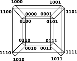
Combinatorics of Cube
We can analyse a cube in pure combinatorics terms, rather than geometric terms, as follows:
| A solid cube represented here as (1..2,1..2,1..2), we can then define subsets of this by making some of the intervals degenerate. | 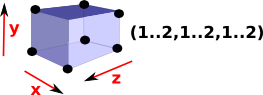 |
From this (1..2,1..2,1..2) cube we can then get the 6 faces by using all possible combinations with one degenerate interval. |
 |
| We can then get the 12 edges by using all possible combinations with two degenerate intervals. | 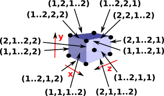 |
We can then get the 8 vertices by using all possible combinations with all three degenerate intervals. |
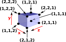 |
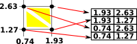
Orientation of a Face
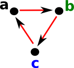
These n-dimensional faces all have orientations. In order to assign directions to the boundary of a face we need to have a consistent set of conventions, for instance, it would help to always start a the same vertex when going around the boundary.
If we are going from (1,1) to (2,2) on this face it should not matter if we go via (1,2) or (2,1) because it commutes. So, on the diagram, we can go 'a' then 'b' or 'c' then 'd', that is: a + b = c + d which gives: a + b - c - d = 0 |
 |
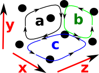
So we need to decide which of these to choose as a positive boundary direction. To do this go back to the earlier notation:
Given a face: [1..2,1..2] To generate the boundary δ[1..2,1..2] we start at the minimum vertex [1,1]
|
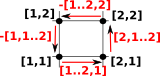 |
So we start at the minimum coordinate indexes, apply the first (non-degenerate) interval, then the second, then minus the first, then minus the second.
The aim of these rules is so that the boundary operator works correctly when the faces are embedded in higher dimensional cubes:
Other Shapes/Spaces as Cubical Complexes
We can construct other common cubical complexes by using CubicalComplexFactory like this:
(22) ->tor := torusSurface()$CubicalComplexFactory

   (22)
         (1..1,1..2,1..1,1..2)
         (1..1,1..2,2..2,1..2)
         (1..1,1..2,1..2,1..1)
         (1..1,1..2,1..2,2..2)
         (2..2,1..2,1..1,1..2)
         (2..2,1..2,2..2,1..2)
         (2..2,1..2,1..2,1..1)
         (2..2,1..2,1..2,2..2)
         (1..2,1..1,1..1,1..2)
         (1..2,1..1,2..2,1..2)
         (1..2,1..1,1..2,1..1)
         (1..2,1..1,1..2,2..2)
         (1..2,2..2,1..1,1..2)
         (1..2,2..2,2..2,1..2)
         (1..2,2..2,1..2,1..1)
         (1..2,2..2,1..2,2..2)
                      Type: FiniteCubicalComplex(Integer)
|
|
For more shapes see page here.
Homology of Cubical Complexes
I have explaind how the homology is implemented on page here.