A square matrix can represent any linear vector translation. Sometimes we want to constrain the elements of the matrix so that it represents a pure solid body rotation. A matrix representation of a rotation therefore contains redundant information, a 3D rotation has 3 degrees of freedom but a 3×3 matrix has 9 scalar values. Provided we restrict the operations that we can do on the matrix then it will remain orthogonolised, for example, if we multiply an orthogonal matrix by orthogonal matrix the result we be another orthogonal matrix (provided there are no rounding errors).
So what are the constraints that we need to apply to a matrix to make sure it is orthogonal? Well there many different ways to define this constraint:
The matrix A is orthogonal if:
- The transpose is equal to the inverse: [A][A]T = [I]
- By making the matrix from a set of mutually perpendicular basis vectors.
- The determinant and eigenvalues are all +1.
- The matrix represents a pure rotation.
These conditions are discussed below:
Transpose and Inverse Equivalence
When we are representing the orientation of a solid object then we want a matrix that represents a pure rotation, but not scaling, shear or reflections. To do this we need a subset of all possible matrices known as an orthogonal matrix.
The matrix A is orthogonal if
[A][A]T = 1
or
[A]-1=[A]T
For information about how to reorthogonalise a matrix see this page.
Orthogonal matrix multiplication can be used to represent rotation, there is an equivalence with quaternion multiplication as described here.
This can be generalized and extended to 'n' dimensions as described in group theory.
Basis vectors
One way to think about a 3x3 orthogonal matrix is, instead of a 3x3 array of scalars, as 3 vectors.
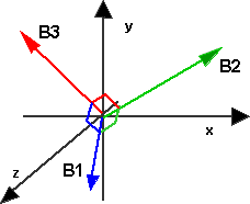
Any point in space can be represented by a linear combination of these vectors.
|
|
= x * |
|
+ y * |
|
+ z * |
|
where:
| B1 = |
|
B2= |
|
B3 = |
|
These basis vectors a mutually perpendicular, so the dot product of any two basis vectors is zero:
B1 • B2 = 0
B2 • B3 = 0
B3 • B1 = 0
Also, if we only know two basis vectors, we can derive the other by using vector cross multiplication, for instance:
B3 = B1 × B2
B1 = B2 × B3
B2 = B3 × B1
Another restriction on the values of the basis vectors is that they are of unit length.
|B1| = B1.x² + B1.y² + B1.z² = 1
|B2| = B2.x² + B2.y² + B2.z² = 1
|B3| = B3.x² + B3.y² + B3.z² = 1
Degrees of Freedom
This matrix has n×n scalar numbers, where n = number of dimensions, in this case 3. But they are not all independent, so although the matrix contains 9 numbers there are less than 9 degrees of freedom. So if we start with 9 degrees of freedom and then apply the three dot product equations we get 6 degrees of freedom, then we apply the three unit length equations we get 3 degrees of freedom.
(We can't also apply the three cross product equations because this is not independent of the other restrictions already applied).
So an orthogonal matrix in 3 dimensions has 3 degrees of freedom as we would expect for a construct which can represent rotations in 3 dimensional space.
'n' Dimensional Orthogonal Matrices
There may not be more than 3 dimensions of space in the physical world? but it can still be useful to look at orthogonal matrices in a way that is independent of the number of dimensions.
We can apply the above rules to an 'n' dimensional orthogonal matrix. We can't use the vector cross product, in dimensions other than 3, to represent mutually perpendicular vectors. However we can still use the dot product of any base vector with a different base vector is zero and the base vectors are unit length. We can derive this from:
B•Bt=[I]
expanding this out:
|
• |
|
= |
|
= |
|
So how many degrees of freedom does an n×n orthogonal matrix have?
We need to know how many independent constraints there are, we can't use both B1•B2=0 and B2•B1=0 because we can derive one from the other.
| B1•B1=1 | B1•B2=0 | B1•B3=0 | B1•B4=0 |
| B2•B2=1 | B2•B3=0 | B2•B4=0 | |
| B3•B3=1 | B3•B4=0 | ||
| B4•B4=1 |
So when we add the first basis vector we have one constraint:
B1•B1=1 (it is unit length)
When we add the second basis vector we have two more constraints:
B2•B2=1 (it is unit length)
B1•B2=0 (B1 and B2 are perpendicular)
When we add the third basis vector we have three more constraints:
B3•B3=1 (it is unit length)
B1•B3=0 (B1 and B3 are perpendicular)
B2•B3=0 (B2 and B3 are perpendicular)
So for an 'n' dimensional matrix the number of degrees of freedom is:
(n-1) + (n-2) + (n-3) … 1
Which is an arithmetic progression as described on this page.
The first term a = n-1
The difference between terms is d = -1
So the sum to n terms is:
Sn = n/2*(2a+(n-1)d)
Sn = n/2*(2(n-1)+(n-1)(-1))
another way to write this is:
n!/(n-2)! 2!
Which is the second entry in pascals triangle, or the number of combinations of 2 elements out of n.
So, using this formula, the degrees of freedom for a given dimension is:
| dimensions 'n' | degrees of freedom |
|---|---|
| 2 | 1 |
| 3 | 3 |
| 4 | 6 |
| 5 | 10 |
| 6 | 15 |
| 7 | 21 |
This is related to bivectors in Geometric Algebra. For a vector of dimension 'n' then the corresponding bivector will have dimension of n!/(n-2)! 2!
So either orthogonal matrices or bivectors might be able to represent:
Determinants of Orthogonal Matrices
All Orthogonal Matrices have determinants of 1 or -1 and all rotation matrices have determinants of 1
For example |R| = cos(a)2 + sin(a)2 = 1
Rotations
When we think about the matrix in this way we can see how a matrix can be used to represent a rotation and to translate to a rotated frame of reference.
For more information about how to use a matrix to represent rotations see here.
Reorthogonalising a matrix
Reorthogonalising a matrix is very important where we doing a lot of calculations and errors can build up, for example where we are recalculating at every frame in an animation as described here.
The following derivation is evolved from this discussion Colin Plumb on newsgroup: sci.math
We want a correction matrix [C] which when multiplied with the original matrix [M] to give an orthogonal matrix [O] such that:
[O] = [C]*[M]
and since [O] is orthogonal then,
[O]-1 = [O]T
combining these equations gives:
[C]*[M] * ([C]*[M])T = [I]
where [I] = identity matrix
as explained here, ([A] * [B])T = [B]T * [A]T so substituting for [C] and [M] gives,
[C]*[M] * [M]T*[C]T = [I]
post multiplying both sides by ([C]T)-1 gives:
[C]*[M] * [M]T = ([C]T)-1
pre multiplying both sides by [C]-1 gives:
[M] * [M]T = [C]-1 ([C]T)-1
If we constrain [C] to be symmetric then [C]T = [C]
[M] * [M]T = [C]-2
[C] = ([M] * [M]T)-(1/2)
So using the taylor series here and using the first two terms we get:
x^(-1/2) = (3-x)/2
So substituting in above gives:
[C] = ([M] * [M]T)-(1/2)
= (3-([M] * [M]T))/2
since we can't subtract a matrix from a scalar I think it should really be written:
[C] = (3[I]-([M] * [M]T))/2
At least this seems to give appropriate results in the examples here.
There are some things about this derivation that make me uneasy, for instance constraining [C] to be symmetric seems to come out of nowhere. This is discussed further on this page.
Orthogonal matrix preserves Inner Product
The orthogonal matrix preserves the angle between vectors, for instance if two vectors are parallel, then they are both transformed by the same orthogonal matrix the resulting vectors will still be parallel.
{v1}•{v2} = [A]{v1} • [A]{v2}
where:
- {v1} = a vector
- {v2} = another vector
- [A] = an orthogonal matrix
- • = the inner or dot product
Eigenvalue of an Orthogonal Matrix
The magnitude of eigenvalues of an orthogonal matrix is always 1.
In other words,
if [A] {v} = λ{v}
then | λ | = 1
As explained here the eigenvalues are the values of λ such that [A] {v} = λ {v}
As a check the determinant is the product of the eigenvalues, since these are all magnitude 1 this checks out.
