Before we can use the scenegraph we need to make the domains available. This is very tedious, it would be better if this was done by default. |
(1) -> )expose SCartesian SCartesian is now explicitly exposed in frame frame1 (1) -> )expose SArgand SArgand is now explicitly exposed in frame frame1 (1) -> )expose SConformal SConformal is now explicitly exposed in frame frame1 (1) -> )expose SceneIFS SceneIFS is now explicitly exposed in frame frame1 (1) -> )expose SceneNamedPoints SceneNamedPoints is now explicitly exposed in frame frame1 (1) -> )expose STransform STransform is now explicitly exposed in frame frame1 (1) -> )expose SBoundary SBoundary is now explicitly exposed in frame frame1 (1) -> )expose ExportXml ExportXml is now explicitly exposed in frame frame1 |
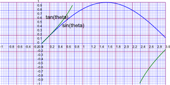
Example 1 - Two dimensional plots with scale.
In this example we have 2 scalar functions superimposed (sine and tangent) plotted in two dimensions. The tangent function has been clipped to values between -1 and +1. The coordinate system is SCartesian(2) which represents two dimensional cartesian coordinates. We also have a grid, numerical axes and text annotation.
DF ==> DoubleFloat
PT ==> SCartesian(2)
fnsin(x:DF):DF == sin(x)
fntan(x:DF):DF == tan(x)
view := boxBoundary(sipnt(-1,-1)$PT,sipnt(3,1)$PT)
sc := createSceneRoot(view)$Scene(PT)
gd := addSceneGrid(sc,view)$Scene(PT)
addSceneRuler(sc,"HORIZONTAL"::Symbol,spnt(0::DF,-0.1::DF)$PT,view)$Scene(PT)
addSceneRuler(sc,"VERTICAL"::Symbol,spnt(-0.1::DF,0::DF)$PT,view)$Scene(PT)
mt1 := addSceneMaterial(sc,3::DF,"blue","green")$Scene(PT)
ln1 := addPlot1Din2D(mt1,fnsin,0..3::DF,49)$Scene(PT)
mt2 := addSceneMaterial(sc,3::DF,"green","green")$Scene(PT)
bb := boxBoundary(sipnt(0,-1)$PT,sipnt(3,1)$PT)
bb2 := addSceneClip(mt2,bb)$Scene(PT)
ln2 := addPlot1Din2D(bb2,fntan,0..3::DF,49)$Scene(PT)
addSceneText(sc,"sin(theta)",32::NNI,_
                   spnt(0.5::DF,0.4::DF)$PT)$Scene(PT)
addSceneText(sc,"tan(theta)",32::NNI,_
                   spnt(0.1::DF,0.6::DF)$PT)$Scene(PT)
writeSvg(sc,"example1.svg") |
|
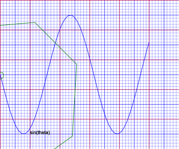
Example 2 - Plotting using complex numbers.
Here the coordinate system is SArgand which represents two dimensions on an argand plane. As we can see the sine function and background grid can be drawn in exactly the same way as with cartesian coordinates. But an exponential function is applied to the tangent function.
DF ==> DoubleFloat
PT ==> SArgand
fnsin(x:DF):DF == sin(x/100::DF)*400::DF
fntan(x:DF):DF == tan(x/100::DF)*400::DF
C ==> Complex DoubleFloat
fnexp(x:C):C == exp(x::C/complex(100::DF,0::DF))
view := boxBoundary(sipnt(0,-500)$PT,sipnt(1200,500)$PT)
sc := createSceneRoot(view)$Scene(PT)
gd := addSceneGrid(sc,view)$Scene(PT)
mt1 := addSceneMaterial(sc,3::DF,"blue","green")$Scene(PT)
ln1 := addPlot1Din2D(mt1,fnsin,0..1000::DF,49)$Scene(PT)
mt2 := addSceneMaterial(sc,3::DF,"green","green")$Scene(PT)
tr2 := addSceneTransform(mt2,stransform(fnexp::(C -> C))_
       )$Scene(PT)
bb := boxBoundary(sipnt(100,-400)$PT,sipnt(1100,400)$PT)
bb2 := addSceneClip(tr2,bb)$Scene(PT)
ln2 := addPlot1Din2D(bb2,fntan,0..1000::DF,49)$Scene(PT)
tx := addSceneText(sc,"sin(theta)",32::NNI,_
       sipnt(200,400)$PT)$Scene(PT)
writeSvg(sc,"example2.svg") |
|
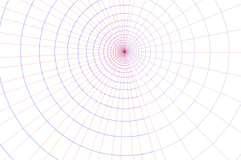
Example 3 - Function of a Complex Number.
Here we use 'addScenePattern1' which consists of horizontal (red) and vertical (blue) lines. We put this under a transform node containing an exponential function which produces the pattern shown here.
DF ==> DoubleFloat
PT ==> SArgand
C ==> Complex DoubleFloat
fnexp(x:C):C == exp(x::C/complex(100::DF,0::DF))
view := boxBoundary(sipnt(0,-500)$PT,sipnt(1200,500)$PT)
sc := createSceneRoot(view)$Scene(PT)
tr2 := addSceneTransform(sc,stransform(fnexp::(C -> C))_
       )$Scene(PT)
gd := addScenePattern(tr2,"GRID"::Symbol,20,view)$Scene(PT)
writeSvg(sc,"example3.svg") |
|
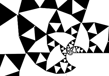
This vertical and horizontal line pattern is useful to test transforms as it indicates whether angles are preserved (lines still meet at right angles) however we can use other test patterns, for instance, this Sierpinski fractel:
DF ==> DoubleFloat
PT ==> SArgand
C ==> Complex DoubleFloat
fnexp(x:C):C == exp(x::C/complex(100::DF,0::DF))
view := boxBoundary(sipnt(0,-500)$PT,sipnt(1200,500)$PT)
sc := createSceneRoot(view)$Scene(PT)
tr2 := addSceneTransform(sc,stransform(fnexp::(C -> C))_
       )$Scene(PT)
gd := addScenePattern(tr2,"SIERPINSKI"::Symbol,4,view)$Scene(PT)
writeSvg(sc,"example32.svg") |
|
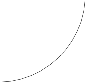
Example 4 - Parametric Two dimensional plot.
Here we use the parametric function sin(t),cos(t) to draw part of a circle.
DF ==> DoubleFloat
PT ==> SCartesian(2)
PPC  ==> ParametricPlaneCurve(DF -> DF)
xsin(t:DF):DF == sin(t)*500::DF
xcos(t:DF):DF == cos(t)*500::DF + 500::DF
view := boxBoundary(sipnt(0,-500)$PT,sipnt(1200,500)$PT)
sc := createSceneRoot(view)$Scene(PT)
tr2 := addSceneTransform(sc,_
       identity()$STransform(PT))$Scene(PT)
gd := addPlot1Din2Dparametric(tr2,curve(xsin,_
                    xcos)$PPC,0..6::DF,49)$Scene(PT)
writeSvg(sc,"example4.svg") |
|
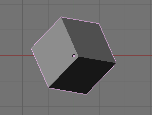
Example 5 - Three Dimensional Box.
Here we have a three dimensional cube which is rotated.
DF ==> DoubleFloat
PT ==> SCartesian(3)
view := boxBoundary(sipnt(0,-500)$PT,sipnt(1200,500)$PT)
sc := createSceneRoot(view)$Scene(PT)
tr2 := addSceneTransform(_
       sc,stransform([[0.7::DF,0.7::DF,0::DF,0::DF],_
                    [-0.7::DF,0.7::DF,0::DF,0::DF],_
                    [0::DF,0::DF,1::DF,0::DF],_
                    [0::DF,0::DF,0::DF,1::DF]]_
                      )$STransform(PT))$Scene(PT)
box := addSceneBox(tr2,1::DF)$Scene(PT)
writeX3d(sc,"example5.x3d") |
|
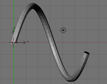
Example 6 - Parametric Three Dimensional plot.
A parametric function, this time in three dimensions.
DF ==> DoubleFloat
PT ==> SCartesian(3)
PSC  ==> ParametricSpaceCurve(DF -> DF)
ysin(t:DF):DF == sin(t)*3::DF
ycos(t:DF):DF == cos(t)*3::DF
ytan(t:DF):DF == t::DF
view := boxBoundary(sipnt(-500,-500)$PT,sipnt(500,500)$PT)
sc := createSceneRoot(view)$Scene(PT)
tr2 := addSceneTransform(sc,_
       identity()$STransform(PT))$Scene(PT)
gd := addPlot1Din3Dparametric(tr2,curve(ysin,_
               ycos,ytan)$PSC,0..(6::DF),49)$Scene(PT)
writeX3d(sc,"example6.x3d") |
|
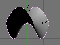
Example 7 - Three Dimensional Surface.
A three dimensional surface.
DF ==> DoubleFloat PT ==> SCartesian(3) xyfn(x:DF,y:DF):DF == x*x-y*y view := boxBoundary(sipnt(0,-500)$PT,sipnt(1200,500)$PT) sc := createSceneRoot(view)$Scene(PT) tr2 := addSceneTransform(sc,identity()$STransform(PT))$Scene(PT) gd := addPlot2Din3D(tr2,xyfn,-1..1,-1..1,49)$Scene(PT) writeX3d(sc,"example7.x3d") |
|
Further Information
A further example on this page here attempts to show, not just how to create an image in FriCAS but also how to use it with other programs.
- User Tutorial on this page.
- Tutorial2 - conformal space.
- User Reference on this page.
- Programmers Reference on this page.
- The code is in file: scene.spad.pamphlet which is available from here.
- Existing Axiom graphics framework on this page.