We can often specify a surface in terms of a set of coordinates (often orthogonal coordinates but cylindrical and spherical coordinates can also be useful). So, for example, a surface of a sphere can be specified by:
r²=x²+y²+z²
We could use this to plot the surface, we might choose to step through two of the dimensions and calculate the third parameter to give a point on the surface of the sphere using:
z = √(r²-x²-y²)
there are possible problems with this:
- Not all values of x,y will produce a point on the sphere.
- Other values of x,y will produce two points corresponding to the front and back faces of the surface.
- Different parts of the surface will be covered in different levels of detail, so the poles will have a much lower density of points than the equator.
In order to minimise these problems it often helps to express the surface in terms of a set of parameters other than the base coordinates:
| Shape |
Parameters |
Limits |
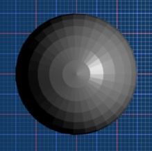
Sphere
r²=x²+y²+z²

|
in spherical coordinates:
c1 = R
c2 = π*u
c3 = 2*π*v
convert to rectangular coordinates
x = c1 * math.sin(c2) * math.cos(c3)
y = c1 * math.sin(c2) * math.sin(c3)
z = c1 * math.cos(c2)
where:
R=1=Sphere Radius |
0< u <1
0< v <1 |
| Cylinder |
|
|
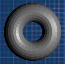
Torus

|
in cylindrical coordinates:
c1 =r0 + r1*cos(2*π*u)
c2 =2*π*v
z =r1*sin(2*π*u)
convert to rectangular coordinates
x = c1 * math.cos(c2)
y = c1 * math.sin(c2)
where:
r0=1=Ring Radius
r1=0.5=Section Radius |
0< u <1
0< v <1 |
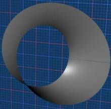
Möbius strip

|
x(u,v) = (1 + (v/2)*cos(u/2))*cos(u)
y(u,v) = (1 + (v/2)*cos(u/2))*sin(u)
z(u,v) = (v/2)*sin(u/2) |
0<u<= 2*π
-1 < v < 1 |
| Klein bottle (represented in 3 dimensions) |
x(u,v) = sin(v)*(4 + 2*cos(u)*cos(t*v)- sin(2*u)*sin(t*v)
y(u,v) = cos(v)*(4 + 2*cos(u)*cos(t*v)- sin(2*u)*sin(t*v)
z(u,v) = 2*cos(u)*sin(t*v)+sin(2*u)*cos(t*v)
t = twist = 0.5
Note1: this is a 'figure-8' Klien bottle. The usual form is built from 4 parts.
Yet another version (Lawson-Klein) can be built from a helicoidal surface.
Note2: This can only be physically realised in four dimensions, since it must pass through itself without making a hole. |
|
Circular helix
|
x=a*sin(t),
y=a*cos(t),
z=at/(2*π*c) |
|
Lissajous curve
|
x= r*sin(theta*t)*cos(phi*t),
y= r*sin(theta*t)*sin(phi*t),
z = cos(phi*t) |
|
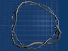
A coil winding around a torus

|
in cylindrical coordinates:
c1=R0 + R1*E0*cos(2*π*n1*v+phi1)+R2*E1*cos(2*π*n2*u+2*π*n1*v+phi1)
c2=2*π*v
z=R1*E0*sin(2*π*n1*v+phi1)+R2*E1*sin(2*pi*n2*u+2*pi*n1*v+phi1)
convert to rectangular coordinates
x = c1 * math.cos(c2)
y = c1 * math.sin(c2)
where:
R1=0.3 = Radius of the section of the torus
R2=0.075 = Radius of the coil
n1=3.3 = Number of full circles of the coil around the torus
phi1 = 0 = Starting angle of the coil
n2= 1= Number of points for the coil section
alpha0=1=Exponential factor for the torus section R1
alpha1=1=Exponential factor for the coil radius R2 |
0< u <1
-2< v <1 |
coil sphere 1
|
in spherical coordinates:
c1=r0+r1t*cos(2*π*u)
c2=(r1t/r0)*sin(2*π*u)+π*v/(2*n)+π/2
c3=2*π*v
convert to rectangular coordinates
x = c1 * math.sin(c2) * math.cos(c3)
y = c1 * math.sin(c2) * math.sin(c3)
z = c1 * math.cos(c2)
where:
r0=1.0=Sphere Radius
r1=0.1=
Coil Max Radius
n=3=Coils
r1t=r1*((abs(v)-n)/n)² |
0< u <1
-n< v <n |
coil sphere 2
|
in spherical coordinates:
c1=r0+r1*tap*cos(2*π*nth*v+thphi)+r2*tap*cos(2*π*u)
c2=r1*tap*sin(2*π*nth*v+thphi)+r2*tap*sin(2*π*u)+π*v/(2*n)+π/2
c3=2*π*v
convert to rectangular coordinates
x = c1 * math.sin(c2) * math.cos(c3)
y = c1 * math.sin(c2) * math.sin(c3)
z = c1 * math.cos(c2)
where:
r0=1.0=Sphere Radius
r1=0.075=Coil Max Radius
r2=0.05=Thread Max Radius
n=3=Coils
nth=6.0=Threads
thphi=0.0=Thread angular offset
tap=((abs(v)-n)/n)² |
0< u <1
-n< v <n |
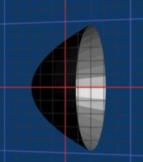
A Paraboloid (Revolution type)
z = a(x²+y²)

|
in cylindrical coordinates:
c1 = u
c2 = 2*π*v
z = a*u²
convert to rectangular coordinates
x = c1 * math.cos(c2)
y = c1 * math.sin(c2)
where:
a=1 |
0< u <1
0< v <1 |
A Paraboloid
z = a(x²+y²)
|
x = u
y = v
z = a*(u²-v²)
where:
a=1 |
-1< u <1
-1< v <1 |
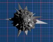
Shell

|
in cylindrical coordinates:
c1 = (r0 + Sp*cos(2*π*u))*E0
c2 = 2*π*v
z = d*E0+Sp*sin(2*π*u)*E0
convert to rectangular coordinates
x = c1 * math.cos(c2)
y = c1 * math.sin(c2)
where:
r0=0.22=Radius of the main winding up coil
r1=0.20=Radius of the circle defining the section
r2=0.5=Spike length
alpha=0.30=Exponential ratio of the spiral
d=-1.10=Vertical displacement of each spiral turn
N0=6=Number of spikes across
M0=8=Sharpness of the spikes across
N1=10.5347=Number of the spikes along (each turn)
M1=12=Sharpness of the spikes across
beta=1.5=Winding of the spikes
a=10=Faloff of spikes
Sp=(r1+r2*Gauss*SpAlong*SpAcross)=Spikes
E0=exp(alpha*v)=Exponential factor
Gauss=exp(-a*(cos(2*π*u)-1.0)²)=Gaussian Spike tapering
SpAlong=((sin(N1*2*π*v)+1)/2.0)M1=Spikes Along formula
SpAcross=((sin(N0*2*π*u+beta*2*π*v)+1)/2.0)M0=Spikes across Formula
|
0< u <1
-9< v <1 |
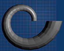
Logarithmic Spiral

|
in cylindrical coordinates:
c1 =r0*E+r1*E*cos(2*π*u)
c2 =2*π*v
z =d*E+r1*E*sin(2*π*u)
convert to rectangular coordinates
x = c1 * math.cos(c2)
y = c1 * math.sin(c2)
where:
r0=1.0=Spiral initial radius
r1=0.25=Bevel initial radius
alpha0=0.15=Exponential factor
d=0.75=Step along z
E=exp(alpha0*2*π*v)=Exponential behavior |
0< u <1
0< v <1 |
