In Euclidean space we often use rectangular (also known as cartesian or orthogonal) coordinates. However in some cases it is often useful to use curvilinear coordinates, we have already seen this for polar, cylindrical and spherical coordinates, this page takes the more general case of curvilinear coordinates.
The curvilinear coordinates have the same number of coordinates as the rectangular coordinates and in order to be able to analyise them in this way there must be a continuous transform from rectangular coordinates and this transform must be reversible so that we can get back to the rectangular coordinates.
Imagine that u¹ ,u² ,u³… represent the curvilinear coordinates of a point. We use superscripts to conform to tensor notation even though there is a danger of confusion with exponents.
We can represent these in terms of rectangular coordinates x, y and z.
So the position of a point in curvilinear coordinates can be represented by P(u¹,u²,u³) in other words a function of the coordinates. The point can also be represented by a function of the rectangular coordinates x, y and z denoted by P(x,y,z)
| coordinate system | representation of point |
|---|---|
| rectangular coordinates | P(x,y,z) |
| curvilinear coordinates | P(u¹,u²,u³) |
We can decompose this function into its components given by the i,j and k basis vectors,
In terms of rectangular coordinates we have:
P(x,y,z) = x e1 + y e2 + z e3
But for curvilinear coordinates we need to use more complex functions:
P(u¹,u²,u³) = X(u¹,u²,u³) e1 + Y(u¹,u²,u³) e2 + Z(u¹,u²,u³) e3
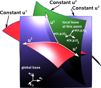
The curvilinear coordinates are intersecting surfaces. If the intersections are all at right angles then the curvilinear coordinates form an orthogonal coordinate system, if not, they form a skew coordinate system.
Local Basis
For the linear case we can express coordinates as a linear equation:
ei Ai = e1 A1 + e2 A2 + e3 A3
For curvilinear coordinates either the basis or the components depend on the location:
e(x,y,z)i Ai = e(x,y,z)1 A1 + e(x,y,z)2 A2 + e(x,y,z)3 A3…
or
ei A(x,y,z)i = e1 A(x,y,z)1 + e2 A(x,y,z)2 + e3 A(x,y,z)3…
where:
- e(x,y,z) is a basis which is a function of position.
- A(x,y,z) are terms which are functions of position.
So we can make the coordinates linear on the very small infinitesimal scale, that is the coordinates tend to linear as the area tends to zero.
Or to turn this argument round: in order to be able to do calculus, that is for the coordinates to be analytic, then the coordinates must be linear on the very small infinitesimal scale.
If we use local basis vectors they can be related to the global coordinate system by two methods:
- they can be built along the coordinate axes (axis-colinear) then the basis vectors transform like covariant vectors.
- they can be built to be perpendicular (normal) to the coordinate surfaces then the basis vectors transform like contravariant vectors.
Tangent
In addition to defining a mapping between rectangular and curvilinear coordinates there is another way to analyse them. For each coordinate we can calculate how much an infinitsimally small piece of space is rotated and scaled (The Kronecker delta is a scale factor) by the coordinate change.
We can calculate the slope or tangent:
| ∂P(u¹,u²,u³) | = | ∂X(u¹,u²,u³) | i + | ∂Y(u¹,u²,u³) | j + | ∂Z(u¹,u²,u³) | k |
| ∂u¹ | ∂u¹ | ∂u¹ | ∂u¹ | ||||
| ∂P(u¹,u²,u³) | = | ∂X(u¹,u²,u³) | i + | ∂Y(u¹,u²,u³) | j + | ∂Z(u¹,u²,u³) | k |
| ∂u² | ∂u² | ∂u² | ∂u² | ||||
| ∂P(u¹,u²,u³) | = | ∂X(u¹,u²,u³) | i + | ∂Y(u¹,u²,u³) | j + | ∂Z(u¹,u²,u³) | k |
| ∂u³ | ∂u³ | ∂u³ | ∂u³ |