Since conformal space is 2 dimensions higher than the space we are working in, that means to model 2D Euclidean space, we need 4D Conformal space. When we model this using geometric algebra we can have bi-vectors, tri-vectors, etc. which gives us upto 16 dimensional quantities in which to represent our various transforms. However we don't need to use all of these because we are dealing with rotations in this 4D space and therefore we only need the even sub-algebra to represent transforms. This consists of 8 numbers, 1 for the scalar, 6 for the bivector and 1 for the pseudo scalar.
Representing Points
We will represent a point at (u,v) in Euclidean space corresponds to the following in conformal space:
-n0+ ½(u²+v²) n∞ + u n1 + v n2
where:
- n0 and n∞ are the basis of the extra 2 dimensions.
- n1 and n1 are the basis of the two dimensional Euclidean space.
- u and v are scalar numbers representing the position in two dimensional space.
The way that these dimension basis vectors combine is derived below and represented as a multiplication table.
This representation of a point has the property that it is a null vector, that is, if we square it we will get zero.
Representing Translations
Transformations are represented as the even sub-algebra, that is scalar and bivector components, like a quaternion. The translation is defined as:
1 + ½(t n∞1 + s n∞2)
where:
- n∞1 is a bivector formed from the n∞ and n1 dimensions.
- n∞2 is a bivector formed from the n∞ and n2 dimensions.
- t and s are scalars representing the components of the translation.
To verify this I have used a free program called Axiom (details here) to do the calculations:
C2 := CliffordAlgebra(4,Expression(Fraction(Integer)),[[0,1,0,0],[1,0,0,0],[0,0,1,0],[0,0,0,1]])
pin := multivector([0,-1,(u*u+v*v)/2,0,u,0,0,0,v,0,0,0,0,0,0,0])$C2
tr := multivector([1,0,0,0,0,0,a1/2,0,0,0,a2/2,0,0,0,0,0])$C2
revtr := reverse(tr)$C2
pout := tr * pin * revtr


             1  2          1  2          1   2   1   2
     - e  + (- v  + a2 v + - u  + a1 u + - a2  + - a1 )e  + (u + a1)e
        1    2             2             2       2      2            3
   +
     (v + a2)e
4 |
Where:
- e1=n0,e2=n∞,e3=n1,e4=n2
which gives:
-n0+ ((u+t)²+(v+s)²) n∞ + 2(u+t) n1 + 2(v+s) n2
So components are individually added as we would expect for translation.
Representing Rotations
Transformations are represented as the even sub-algebra, that is scalar and bivector components, like a quaternion. The rotation is defined as:
cos(θ/2) + sin(θ/2) n12
where:
- n12 is a bivector formed from the n1 and n2 dimensions.
- θ is a scalar representing the angle of rotation.
To verify this I have used a free program called Axiom (details here) to do the calculations:
theta : Expression(DoubleFloat)
c:Expression(DoubleFloat) := cos(theta/2)
s:Expression(DoubleFloat) := sin(theta/2)
pin := multivector([0,-1,(u*u+v*v)/2,0,u,0,0,0,v,0,0,0,0,0,0,0])$C2
tr := multivector([c,0,0,0,0,0,0,0,0,0,0,0,s,0,0,0])$C2
revtr := reverse(tr)$C2
pout := tr * pin * revtr
                          2                     2
     (- 1.0 sin(0.5 theta)  - 1.0 cos(0.5 theta) )e
                                                   1
   +
            2        2               2         2        2               2
     ((0.5 v  + 0.5 u )sin(0.5 theta)  + (0.5 v  + 0.5 u )cos(0.5 theta) )e
                                                                           2
   +
                               2
         - 1.0 u sin(0.5 theta)  + 2.0 v cos(0.5 theta)sin(0.5 theta)
       +
                         2
         u cos(0.5 theta)
    *
       e
        3
   +
                               2
         - 1.0 v sin(0.5 theta)  - 2.0 u cos(0.5 theta)sin(0.5 theta)
       +
                         2
         v cos(0.5 theta)
    *
       e
4 |
Where:
- e1=n0,e2=n∞,e3=n1,e4=n2
So substituting: sin² + cos² =1 gives:
-e1  +(0.5 v²  + 0.5 u² )e2
- 1.0 u sin(0.5 theta)²  + 2.0 v cos(0.5 theta)sin(0.5 theta)
+ u cos(0.5 theta)²*e3
- 1.0 v sin(0.5 theta)²  - 2.0 u cos(0.5 theta)sin(0.5 theta)
+ v cos(0.5 theta)²*e4
and substititing double angle formula:
sin(2A) = 2 sin A cos A and cos(2A) = cos²A - sin²A gives:
-e1  +0.5 (v² + u²)e2
+ u cos(theta) + v sin(theta)*e3
+ v cos(theta) - u sin(theta)*e4
Scaling
Transformations are represented as the even sub-algebra, that is scalar and bivector components, like a quaternion. Scaling is defined as:
cosh(γ/2) + sinh(γ/2) n0∞
where:
- n0∞ is a bivector formed from the origin and infinity dimensions.
- γ is a scalar representing a scale factor of eγ .
To verify this I have used a free program called Axiom (details here) to do the calculations:
gamma : Expression(DoubleFloat)
ch:Expression(DoubleFloat) := cosh(gamma/2)
sh:Expression(DoubleFloat) := sinh(gamma/2)
pin := multivector([0,-1,(u*u+v*v)/2,0,u,0,0,0,v,0,0,0,0,0,0,0])$C2
tr := multivector([ch,0,0,sh,0,0,0,0,0,0,0,0,0,0,0,0])$C2
revtr := reverse(tr)$C2
pout := tr * pin * revtr
                              2
         - 1.0 sinh(0.5 gamma)  - 2.0 cosh(0.5 gamma)sinh(0.5 gamma)
       +
                              2
         - 1.0 cosh(0.5 gamma)
    *
       e
        1
   +
               2        2                2
         (0.5 v  + 0.5 u )sinh(0.5 gamma)
       +
                 2        2
         (- 1.0 v  - 1.0 u )cosh(0.5 gamma)sinh(0.5 gamma)
       +
               2        2                2
         (0.5 v  + 0.5 u )cosh(0.5 gamma)
    *
       e
        2
   +
                             2                    2
     (- 1.0 u sinh(0.5 gamma)  + u cosh(0.5 gamma) )e
                                                     3
   +
                             2                    2
     (- 1.0 v sinh(0.5 gamma)  + v cosh(0.5 gamma) )e
4 |
Where:
- e1=n0,e2=n∞,e3=n1,e4=n2
So substituting: cosh² - sinh² = 1 and substititing double angle formula:
sinh(2A) = 2 sinh A cosh A and = cosh(2A) = cosh²A + sinh²A gives:
(-cosh(gamma)-sinh(gamma))e1  +(0.5 v² + 0.5 u²)(-sinh(gamma)+cosh(gamma)) e2
+ u e3 + v e4
So substituting: cosh² - sinh² = 1 again gives:
(-cosh(gamma)-sinh(gamma))e1 +(0.5 v² + 0.5 u²) e2 + u e3 + v e4
Which, when re-normalised, scales the points by a factor of: eγ = cosh(γ)+sinh(γ)
Reflection in origin
A special case of scaling is caling is reflection in origin which is represented by a transform of:
n0∞
where:
- n0∞ is a bivector formed from the origin and infinity dimensions.
To verify this I have used a free program called Axiom (details here) to do the calculations:
pin := multivector([0,-1,(u*u+v*v)/2,0,u,0,0,0,v,0,0,0,0,0,0,0])$C2
tr := multivector([0,0,0,1,0,0,0,0,0,0,0,0,0,0,0,0])$C2
revtr := reverse(tr)$C2
pout := tr * pin * revtr
                         2        2
   (5)  - 1.0 e  + (0.5 v  + 0.5 u )e  - 1.0 u e  - 1.0 v e
1 2 3 4 |
Reflection in unit circle
To reflect in a unit circle we use a transform of:
n0 - ½n∞
where:
- n0 is the point at the origin.
- n∞ is the point at infinity.
To verify this I have used a free program called Axiom (details here) to do the calculations:
pin := multivector([0,-1,(u*u+v*v)/2,0,u,0,0,0,v,0,0,0,0,0,0,0])$C2
tr := multivector([0,1,-0.5,0,0,0,0,0,0,0,0,0,0,0,0,0])$C2
revtr := reverse(tr)$C2
pout := tr * pin * revtr
          2    2
   (5)  (v  + u )e  - 0.5 e  + u e  + v e
1 2 3 4 |
This reverses the n0 and n∞ components. When we re-normalise we get:
-n0 + 0.5/(v²+u²) n∞+ u/(v²+u²) n1+ v/(v²+u²) n2
Reflection in circle radius eγ
We do this by scaling to unit by e-γ then reflect then scale back to eγ. so we need to multiply the following together:
(cosh(-γ/2) + sinh(-γ/2) n0∞)(n0 - ½n∞)(cosh(γ/2) + sinh(γ/2) n0∞)
applying symmetric and anti-symmetric properties from this page gives:
(cosh(γ/2) - sinh(γ/2) n0∞)(n0 - ½n∞)(cosh(γ/2) + sinh(γ/2) n0∞)
To calculate this I have used a free program called Axiom (details here) to do the calculations:
gamma : Expression(DoubleFloat)
ch:Expression(DoubleFloat) := cosh(gamma/2)
sh:Expression(DoubleFloat) := sinh(gamma/2)
tr1 := multivector([ch,0,0,-sh,0,0,0,0,0,0,0,0,0,0,0,0])$C2
tr2 := multivector([0,1,-0.5,0,0,0,0,0,0,0,0,0,0,0,0,0])$C2
tr3 := multivector([ch,0,0,sh,0,0,0,0,0,0,0,0,0,0,0,0])$C2
tr1*tr2*tr3
                          2
           sinh(0.5 gamma)  - 2.0 cosh(0.5 gamma)sinh(0.5 gamma)
         +
                          2
           cosh(0.5 gamma)
    *
       e
        1
   +
                              2
         - 0.5 sinh(0.5 gamma)  - 1.0 cosh(0.5 gamma)sinh(0.5 gamma)
       +
                              2
         - 0.5 cosh(0.5 gamma)
    *
       e
2 |
applying sinh(2A) = 2 sinh A cosh A and = cosh(2A) = cosh²A + sinh²A gives:
(cosh(gamma) - sinh(gamma)) n0 - 0.5( cosh(gamma) + sinh(gamma)) n∞
Reflection in Plane
To reflect in a plane we use a transform of:
a1 n1 + a2 n2
where:
- n1and n2 are basis vectors.
- since we only need the derection of the plane through the origin then a1 and a2 form a unit length vecter. That is a2² + a1² = 1
To verify this I have used a free program called Axiom (details here) to do the calculations:
pin := multivector([0,-1,(u*u+v*v)/2,0,u,0,0,0,v,0,0,0,0,0,0,0])$C2
tr := multivector([0,0,0,0,a1,0,0,0,a2,0,0,0,0,0,0,0])$C2
revtr := reverse(tr)$C2
pout := tr * pin * revtr
        2     2                2         2  2            2         2  2
     (a2  + a1 )e  + ((- 0.5 a2  - 0.5 a1 )v  + (- 0.5 a2  - 0.5 a1 )u )e
                 1                                                       2
   +
                             2     2            2         2
     (2.0 a1 a2 v + (- 1.0 a2  + a1 )u)e  + ((a2  - 1.0 a1 )v + 2.0 a1 a2 u)e
                                        3                                    4
|
Applying a2² + a1² = 1 gives:
n0 - 0.5 (v² + u² )n∞ + (2.0 a1 a2 v + (-a2² + a1² )u)n1 + ((a2² - a1² )v + 2.0 a1 a2 u)n2
Normalising (multiply by -1) gives:
-n0 + 0.5 (v² + u² )n∞ + (-2.0 a1 a2 v + (a1²-a2² )u)n1 + ((a1² - a2² )v - 2.0 a1 a2 u)n2
Concatenating Transforms
When using quaternions and matricies we can combine translations by multiplying them together, we can do the same in conformal space:
If we first apply a translation of t1:
(1 + ½ t1 n∞1)
Then we apply a subsequent translation of t2:
(1 + ½ t2 n∞1)
The equivalent translation will be:
(1 + ½ t2 n∞1)*(1 + ½ t1 n∞1)
=(1 + ½ t2 n∞1 + ½ t1 n∞1+ ¼ t1t2 n∞1∞1)
The last product is zero (see table at bottom) so the result is:
=1 + ½(t2+t1) n∞1
which is what we would expect.
Derivation of the Algebra
The result of multiplying the various basis vectors are shown at the bottom of this page
Representing Transforms
This can be used to represent the group of spatial displacements in two dimensions SE(2) which can be used to represent a combination of 2D rotation and displacement.
The advantage of this is that we can represent a combined rotation with displacement operation with one multiplication operation.
- The 1 and n12 terms together can represent rotation (as a normalised complex number).
- The n∞1 + n∞2 terms together can represent displacement.
In order to investigate the practicality of this we can try to use it in the car racing game (which is developed on these pages). This is used in the following examples:
Example 1 - Pure Displacement (no rotation)
The representation of a point is given by:
|
= |
|
So if we are initially at point (u=3, v=4) this will be represented by the vector:
|
= |
|
= |
|
We now want to displace this by (x=4, y=3) this will be represented by the even multivector (scalar + bivector):
|
= |
|
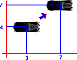
So to combine these, to give the resulting position, we multiply together their representations using sandwich product:
(1 + 2 n∞1 + 1.5 n∞2)*(- n0 + 25 n∞ +6 n1 + 8 n2)*(1 -2 n∞1 -1.5 n∞2)
Multiplying out the terms using the multiplication table at the bottom of this page we get:
= -n0 +98 n∞ +14 n1 +14 n2
since:
|
= |
|
= |
|
u = 7
v = 7
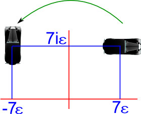
Example 2 - Pure Rotation (no displacement)
Lets take the example of a rotation by 180° this is represented by:
(0 + 1 n12)
So to combine these, to give the resulting position, we multiply together their representations using sandwich product:
(0 + 1 n12)*(-1 n0 + 25 n∞ +6 n1 + 8 n2)*(0 - 1 n12)
= n12*(-1 n0 + 25 n∞ +6 n1 + 8 n2)*(-n12)
= (-1 (n012) + 25 (n∞12) +6 (-n2) + 8 (n1))*(-n12)
= -(-1 (-n0) + 25 (-n∞) -6 (-n1) + 8 (n2))
=-1 n0 + 25 n∞ -6 n1 - 8 n2
since:
|
= |
|
u = -3
v = -4
so (0 + 1 n12) rotates by 180°.
Example - Combined Displacement and Rotation
Starting from the previous position:
(-n0+ 98 n∞ + 14 n1+ 14 n2)
and applying a rotation of 90 represented by:
(0.7071 + 0.7071 n12)
We combine them by multiplying as before:
(0.7071 + 0.7071 n12)*(-n0+ 98 n∞ + 14 n1+ 14 n2)*(0.7071 - 0.7071 n12)
=0.7071*(-n0+ 98 n∞ + 14 n1+ 14 n2 -n12n0+ 98n12 n∞ + 14 n12n1+ 14 n12n2)*(0.7071 - 0.7071 n12)
multiplying out the terms using the multiplication table at the bottom of this page we get:
=0.7071*(-n0+ 98 n∞ + 14 n1+ 14 n2 -n012+ 98 n∞12 - 14 n2+ 14 n1)*(0.7071 - 0.7071 n12)
=-n0+ 98 n∞ + 14 n1- 14 n2
So we can see that the object is rotated about the origin.
We could have produced the same result by combining the rotation and translation operators into a single operator:
(0.7071 + 0.7071 n12) * (1 + 2 n∞1 + 1.5 n∞2)
= 0.7071(1 + n12) * (1 + 2 n∞1 + 1.5 n∞2)
= 0.7071(1 + 2 n∞1 + 1.5 n∞2+ n12 + 2 n12n∞1 + 1.5 n12n∞2)
= 0.7071(1 + 2 n∞1 + 1.5 n∞2+ n12 - 2 n∞2+ 1.5 n∞1)
= 0.7071(1 + 3.5 n∞1 -0.5 n∞2+ n12)
then we can apply this operator to the original point (u=3, v=4) using the sandwich product.
0.7071(1 + 3.5 n∞1 -0.5 n∞2+ n12)(- n0 + 25 n∞ +6 n1 + 8 n2)0.7071(1 - 3.5 n∞1 +0.5 n∞2- n12)
= 0.5(1 + 3.5 n∞1 -0.5 n∞2+ n12)*(- n0 + 25 n∞ +6 n1 + 8 n2)*(1 - 3.5 n∞1 +0.5 n∞2- n12)
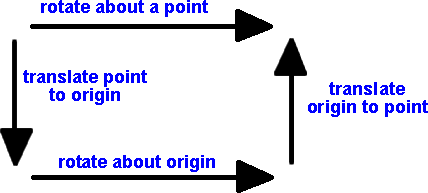
Rotation about a point
In the above we are rotating about the origin. This is sometimes what we want to do, for instance, if we are observing the world from the frame of reference of a car and we assume it to be at the origin then, when it turns, the other cars will appear to rotate round it. If we want a car to rotate about its own centre then we can just multiply the n1 and n2 part and ignore the n0 and n∞ part.
If we want to rotate about an arbitrary point then we first translate this point to the origin, then rotate about the origin, then translate the origin back to the point (as discussed on this page).
Inverse of multivector
Due to the zero terms in the multiplication table I don't think there is a general multiplicative inverse because information is lost by multiplication.
However, if we restrict ourselves to the linear rotation-displacement discussed above, then there must be an inverse because the operations they represent have an inverse. The complex number is always normalised so its inverse will be its conjugate and the inverse of the displacement is minus its value.
So, in this case, the inverse of:
1 +4 n∞1 +3 n∞2
is:
1 -4 n∞1 -3 n∞2
Complete Multiplication (Cayley) Table For This Case
This table could have been generated from basis vectors as e1,e2,e3 and e4
where:
- e1,e2 and e3 square to positive
- e4 squares to negative
Then converting to alternative basis vectors which allow us to represent our space in terms of null vectors as n1,n2,n3 and n4
where:
- n1,n2 square to positive
- n3,n4 square to zero
so they relate to each other as:
n1= e1
n2= e2
n3= e3 + e4
n4= e3 - e4
This would be tedious to do so I have used a free program called Axiom (details here) to do the calculations:
)set output html on C2 := CliffordAlgebra(4,Expression(DoubleFloat),[[0,1,0,0],[1,0,0,0],[0,0,1,0],[0,0,0,1]]) toTable(*)$C2 |