Introduction
In Axiom/FriCAS there are various domains, such as Integer and Float, and these have literal values and operations on their values. However, if Axiom/FriCAS is to be more than a sophisticated calculator, we need variables that can represent elements of these domains.
Expression is defined over a domain and allows us to represent variables and various functions.
In some sense this puts Expression at the heart of Axiom/FriCAS and it explains a lot about what Axiom/FriCAS is good at and what it is not so good at. I therefore think it is important to understand the Expression domain.
An algebra tends to be represented by a set of binary and unary operations. These are closed operations. |
|
In order to represent expressions, that is an algebra with variables, we have the Expression structure over that algebra, this is an open tree structure.
Expression
How should expression be represented? As far as I know there is no canonical form, there is no general algorithm to decide if two expression represent the same value and theorem of Richardson says that problem of deciding if an expression is zero is un-decidable.
So the best we can do is choose a representation that is efficient most of the time and is a reasonable compromise.
As an example lets take the expression: x+sin(x)²+sin(y)²
| Since we allow variables then our algebra becomes a recursive tree structure. Perhaps the most natural way to represent this would be to make each operator a separate node in the tree and the variables and literals being the leaves: |  |
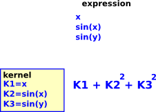
However 'Expression' in Axiom/FriCAS represents this differently. '+','-' and '*' operators are combined into a polynomial. This multi-variable (multivariate) polynomial is defined over 'kernels'. A kernel is a variable or function of an expression (treated like it is an undivided element). So we still have a tree structure but this time in terms of polynomials. The idea is that expressions form a field and kernels give generators of that field over base ring. |
 |
Representing Expressions
How do we efficiently encode instances of these expressions? First we look at how its components are encoded:
| Domain | Encoding | |||||||||
|---|---|---|---|---|---|---|---|---|---|---|
SparseUnivariatePolynomial example: x+3*x2+5*x4 |
This is represented by a list of pairs: The exponent value and the scalar multiplier for the term. It is 'sparse' because terms with zero multipliers do not need to be included. The name of the variable does not need to be included. Rep := List Record(k:NNI,c:R) |
|||||||||
SparseMultivariatePolynomial example: |
Polynomials of many variables are defined recursivly in terms of polynomials of one variable. Rep := Union(R, VPoly) |
|||||||||
| Kernel | ||||||||||
| Expression | if R is Ring then Rep := MP( R,Kernel %) where MP= SparseMultivariatePolynomial |
(1) -> e:Expression(Float) := x + sin(x)^2 + sin(y)^2

              2         2
   (1)  sin(y)  + sin(x)  + x
                                                      Type: Expression(Float)
(3) -> k2:Kernel(Expression(Float)) := mainKernel(e)

   (3)  sin(y)
                                              Type: Kernel(Expression(Float))
(4) -> k3:=kernels([e])

   (4)  [sin(y),sin(x),x]
                                        Type: List(Kernel(Expression(Float)))
(5) -> e::SparseMultivariatePolynomial(Float,Kernel(Expression(Float)))

   Cannot convert from type Expression(Float) to
      SparseMultivariatePolynomial(Float,Kernel(Expression(Float))) for
      value
         2         2
   sin(y)  + sin(x)  + x
(9) -> SMP3 := SparseMultivariatePolynomial(Float,K3)
 (9)  SparseMultivariatePolynomial(Float,OrderedVariableList([x,y]))
    Type: Type
    (10) -> e::SMP3

    Cannot convert from type Expression(Float) to
    SparseMultivariatePolynomial(Float,OrderedVariableList([x,y]))
    for value
    2         2
    sin(y)  + sin(x)  + x


(1) -> SMP5 := SparseMultivariatePolynomial(Integer,OrderedVariableList([x,y]))

   (1)  SparseMultivariatePolynomial(Integer,OrderedVariableList([x,y]))
                                                                   Type: Type
(2) -> e5:Expression(Integer) := 2*x + 3*x^2 + 4*y^2

          2     2
   (2)  4y  + 3x  + 2x
                                                    Type: Expression(Integer)
(3) -> e5 pretend SMP5


   >> System error:
   The value
  (1 #S(SPAD-KERNEL :OP #(|y| 0 (((|%symbol|)))) :ARG NIL :NEST 1) (2 0 . 4)
   (0 1 #S(SPAD-KERNEL :OP #(|x| 0 (((|%symbol|)))) :ARG NIL :NEST 1) (2 0 . 3)
    (1 0 . 2)))
is not of type
  FIXNUM.

(3) -> e6:Expression(Integer) := 2*x + 3*x^2 + 4*y^2 + 5*x*y

          2            2
   (3)  4y  + 5x y + 3x  + 2x
                                                    Type: Expression(Integer)
(4) -> e6 pretend SMP5


   >> System error:
   The value
  (1 #S(SPAD-KERNEL :OP #(|y| 0 (((|%symbol|)))) :ARG NIL :NEST 1) (2 0 . 4)
   (1 1 #1=#S(SPAD-KERNEL :OP #(|x| 0 (((|%symbol|)))) :ARG NIL :NEST 1)
    (1 0 . 5))
   (0 1 #1# (2 0 . 3) (1 0 . 2)))
is not of type
  FIXNUM.

(4) ->
(note: FIXNUM means integer in lisp) |
SparseMultivariatePolynomial
MultivariatePolynomial
This type is the basic representation of sparse recursive multivariate ++ polynomials whose variables are from a user specified list of symbols. ++ The ordering is specified by the position of the variable in the list. ++ The coefficient ring may be non commutative, ++ but the variables are assumed to commute.
MultivariatePolynomial(vl : List Symbol, R : Ring)
   ==  SparseMultivariatePolynomial(--SparseUnivariatePolynomial,
R, OrderedVariableList vl) |
SparseMultivariatePolynomial
This type is the basic representation of sparse recursive multivariate polynomials. It is parameterized by the coefficient ring and the variable set which may be infinite. The variable ordering is determined by the variable set parameter. The coefficient ring may be non-commutative, but the variables are assumed to commute.
(1) -> MP1 := SparseMultivariatePolynomial(Integer,OrderedVariableList([x,y]))

   (1)  SparseMultivariatePolynomial(Integer,OrderedVariableList([x,y]))
                                                                   Type: Type
(2) -> e1:MP1 := x

   (2)  x
       Type: SparseMultivariatePolynomial(Integer,OrderedVariableList([x,y]))
(3) -> e2:MP1 := y

   (3)  y
       Type: SparseMultivariatePolynomial(Integer,OrderedVariableList([x,y]))
(4) -> e3 := 2*e1 + 3*e1^2 + 4*e2^2 + 5*e1*e2

          2                 2
   (4)  3x  + (5y + 2)x + 4y
       Type: SparseMultivariatePolynomial(Integer,OrderedVariableList([x,y]))
(5) -> coefficients(e3)

   (5)  [3,5,2,4]
                                                          Type: List(Integer)
(6) -> leadingMonomial(e3)

          2
   (6)  3x
       Type: SparseMultivariatePolynomial(Integer,OrderedVariableList([x,y]))
(7) -> monomials(e3)

           2           2
   (7)  [3x ,5y x,2x,4y ]
 Type: List(SparseMultivariatePolynomial(Integer,OrderedVariableList([x,y])))
(8)-> e3

          2                 2
   (8)  3x  + (5y + 2)x + 4y
       Type: SparseMultivariatePolynomial(Integer,OrderedVariableList([x,y]))
(9) -> variables(e3)

   (9)  [x,y]
                                       Type: List(OrderedVariableList([x,y]))
|
SparseUnivariatePolynomial
This domain represents univariate polynomials over arbitrary (not necessarily commutative) coefficient rings. The variable is unspecified so that the variable displays as on output.
If it is necessary to specify the variable name, use type UnivariatePolynomial.
The representation is sparse in the sense that only non-zero terms are represented.
Note: if the coefficient ring is a field, this domain forms a euclidean domain.
Constructing:
fmecg(p1:%, e:NonNegativeInteger, r:R,p2:%)
represents: p1 - r * X^e * p2
where:
- p1:%
- e:NonNegativeInteger - exponent
- r:R - multipier
- p2:%
(2) -> Z := 0$SparseUnivariatePolynomial(Integer)

   (2)  0
                                    Type: SparseUnivariatePolynomial(Integer)
(3) -> One := 1$SparseUnivariatePolynomial(Integer)

   (3)  1
                                    Type: SparseUnivariatePolynomial(Integer)
(4) -> A := fmecg(Z,3,4,One)$SparseUnivariatePolynomial(Integer)

            3
   (4)  - 4?
                                    Type: SparseUnivariatePolynomial(Integer)
(5) -> B := fmecg(A,2,1,One)$SparseUnivariatePolynomial(Integer)

            3    2
   (5)  - 4?  - ?
                                    Type: SparseUnivariatePolynomial(Integer)
(6) -> C := fmecg(A,2,1,B)$SparseUnivariatePolynomial(Integer)

          5    4     3
   (6)  4?  + ?  - 4?
Type: SparseUnivariatePolynomial(Integer) |
Diagram
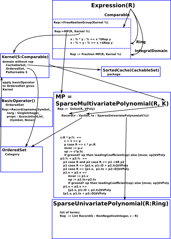
This diagram is a (not very successful) attempt to put all this complex information into one diagram.

Information from WaldekSee this thread "bad reduction" is standard terminology. PGCD works by treating multivariate polynomials as polynomials in one variable (called main variable) with coefficients beeing polynomials in other (auxiliary) variables. PGCD chooses random values for auxiliary variables and substitutes them into arguments. Then in tries to reconstruct multivariate GCD from GCD of univariate images. There are various obstacles to this, if they happen we speak about bad reduction. If bad reduction is detected PGCD should try different evaluation point. What I wrote above is standard background explained in papers about polynomial GCD. If you did not know this, then IMHO searching for information is appropriate action. Once you accept randomized nature of PGCD it should be clear that repeating test is a method to increase probability of hitting the bug. You could easily check what was wrong by running the code, it requires less effort than writing the message to the list. The error is: >> Error detected within library code: which means that division which code expected to be exact failed. Looking at change in 'lift' function you will notice that instead of coercing result of division to SUP I first check for "failed" and in such case return "failed" from 'lift'. I coerce only when division was exact. From this alone it should be clear that we get different behaviour only in case when old code was wrong (produced runtime error). The testcase shows that such cases do happen. It is easy to prove that in case of good reduction division is always exact. So the new failing cases are all bad reductions. Since 'lift' should fail in case of bad reduction this is correct behaviour. |